Particle-Particle Particle-Mesh Algorithm#

The Particle-Particle Particle-Mesh (PPPM or P3M) algorithm is a Fourier-based Ewald summation method formulated by Hockney and Eastwood in the late 1980s.

Ewald Sum#

The Ewald summation is a method to compute the potential energy of long-range interaction in periodic systems. More details can be found in this Wikipedia article. In the following we will concentrate on explaining how it is used in the context of Sarkas.

Long range forces are calculated using the Ewald method which consists in dividing the potential into a short and a long range part. Physically this is equivalent to adding and subtracting a screening cloud around each charge. This screening cloud is usually chosen to be given by a Gaussian charged density distribution, but it need not be. The primary reason for choosing a Gaussian is its spherical symmetry. In the following we will calculate the charge density with its surrounding clouds and the corresponding energy density of each.

Total charge density#

Consider a system of \(N\) randomly distributed charges whose distribution is given by

\[\rho_N ( \mathbf r) = \sum_{i = 1}^{N} q_i \delta( \mathbf r - \mathbf r_i).\]

At each point \(\mathbf r_i\) we add and substract a Gaussian screening cloud

\[\rho_S (\mathbf r) = -\frac{q_i \alpha^{3/2}}{\pi} e^{-\alpha^2 (\mathbf r - \mathbf r_i)^2}.\]

The total charge density at point \(\mathbf r\) is then

\[\rho(\mathbf r) = \sum_{i}^N \left \{ \left ( q_i\delta( \mathbf r - \mathbf r_i) - \frac{q_i\alpha^{3/2}}{\pi} e^{-\alpha^2 \left( \mathbf r - \mathbf r_i \right )^2 } \right ) + \frac{q_i\alpha^{3/2}}{\pi} e^{-\alpha^2 \left( \mathbf r- \mathbf r_i \right )^2 } \right \},\]

where, again, the first term is the charge density due to the real particles and the last two terms are the negative and positive screening clouds. The first two terms are in parenthesis to emphasizes the splitting into

\[\rho(\mathbf r) = \rho_{\mathcal R}(\mathbf r) + \rho_{\mathcal F}(\mathbf r)\]

\[\rho_{\mathcal R} (\mathbf r) = \sum_{i}^N \left ( q_i\delta( \mathbf r- \mathbf r_i) - \frac{q_i\alpha^{3/2}}{\pi} e^{-\alpha^2 \left( \mathbf r- \mathbf r_i \right )^2 } \right ), \quad \rho_{\mathcal F}(\mathbf r) = \sum_{i}^N \frac{q_i\alpha^{3/2}}{\pi} e^{-\alpha^2 \left( \mathbf r- \mathbf r_i \right )^2 }\]

where \(\rho_{\mathcal R}(\mathbf r)\) indicates the charge density leading to the short range part of the potential and \(\rho_{\mathcal F}(\mathbf r)\) leading to the long range part. The subscripts \(\mathcal R, \mathcal F\) stand for Real and Fourier space indicating the way the calculation will be done.

The potential at every point \(\mathbf r\) is calculated from Poisson’s equation

\[-\nabla^2 \phi( \mathbf r) = 4\pi \rho_{\mathcal R} (\mathbf r) + 4\pi \rho_{\mathcal F}( \mathbf r).\]

Short-range term#

The short range term is calculated in the usual way

\[-\nabla^2 \phi_{\mathcal R}( \mathbf r) = 4\pi \sum_{i}^N \left ( q_i\delta( \mathbf r- \mathbf r_i) - \frac{q_i\alpha^{3/2}}{\pi} e^{-\alpha^2 \left( \mathbf r- \mathbf r_i \right )^2 } \right ).\]

The first term \(\delta(\mathbf r - \mathbf r_i)\) leads to the usual Coulomb potential (\(\sim 1/r\)) while the Gaussian leads to the error function

\[\phi_{\mathcal R}( \mathbf r ) = \sum_i^N \frac{q_i}{r} - \frac{q_i}{r}\text{erf} (\alpha r) = \sum_i^N \frac{q_i}{r} \text{erfc}(\alpha r)\]

(eq:phi_R)

Long-range term#

The long range term is calculated in Fourier space

\[k^2 \tilde\phi_{\mathcal F}(k) = 4\pi \tilde\rho_{\mathcal F}(k)\]

where

\[\tilde\rho_{\mathcal F}(k) = \frac{1}{V} \int d\mathbf re^{- i \mathbf k \cdot \mathbf r} \rho_{\mathcal F}( \mathbf r ) = \sum_{i}^N \frac{q_i\alpha^{3/2}}{\pi V} \int d\mathbf r e^{- i \mathbf k \cdot \mathbf r} e^{-\alpha^2 \left( \mathbf r - \mathbf r_i \right )^2 } = \sum_{i}^N \frac{q_i}{V} e^{-i \mathbf k \cdot \mathbf r_i} e^{-k^2/(4\alpha^2)}.\]

The potential is then

\[\tilde \phi_{\mathcal F}(\mathbf k) = \frac{4\pi}{k^2} \frac{1}{V} \sum_{i}^N q_i e^{-i\mathbf k \cdot \mathbf r_i} e^{-k^2/(4\alpha^2)} = \frac{1}{V} \sum_i^N v(k)e^{-k^2/(4 \alpha^2)} q_i e^{-i \mathbf k \cdot \mathbf r_i}\]

and in real space

\[\phi_{\mathcal R}( \mathbf r ) = \sum_{\mathbf k \neq 0} \tilde \phi_{\mathcal F}(\mathbf k)e^{i \mathbf k \cdot \mathbf r} = \frac{1}{V} \sum_{\mathbf k\neq 0} \sum_{i}^N v(k) e^{-k^2/(4\alpha^2)}q_i e^{i \mathbf k \cdot ( \mathbf r- \mathbf r_i) },\]

(eq:U_R)

where the \(\mathbf k = 0\) is removed from the sum because of the overall charge neutrality.

The potential energy created by this long range part is

\[U_{\mathcal F} = \frac {1}{2} \sum_i^N q_i \phi_{\mathcal F}(\mathbf r_i) = \frac{1}{2} \frac{1}{V} \sum_{i,j}^N q_i q_j \sum_{\mathbf k \neq 0 } v(k) e^{-k^2/(4\alpha^2)}e^{i \mathbf k \cdot ( \mathbf r_i - \mathbf r_j) } = \frac{1}{2} \sum_{\mathbf k \neq 0} |\rho_0(\mathbf k)|^2 v(k) e^{-k^2/(4\alpha^2)},\]

(eq:U_F)

where I used the definition of the charge density

\[\rho_0(\mathbf k) = \frac 1V \sum_i^N q_i e^{i \mathbf k \cdot \mathbf r_i}.\]

However, in the above sum we are including the self-energy term, i.e. \(\mathbf r_i = \mathbf r_j\). This term can be easily calculated and then removed from \(U_{\mathcal F}\)

\[\frac{\mathcal Q^2}{2V} \sum_{\mathbf k} \frac{4\pi}{k^2} e^{-k^2/(4\alpha^2)} \rightarrow \frac{\mathcal Q^2}{2V} \left ( \frac{L}{2\pi} \right )^3 \int dk (4\pi)^2 e^{-k^2/(4\alpha^2) } = \mathcal Q^2 \frac{(4\pi)^2}{2V} \left ( \frac{L}{2\pi} \right )^3 \sqrt{\pi } \alpha = \mathcal Q^2 \frac{\alpha}{\sqrt{\pi} }\]

where \(\mathcal Q^2 = \sum_i^N q_i^2\), note that in the integral we have re-included \(\mathbf k = 0\), but this is not a problem. Finally the long-range potential energy is

\[U_{\mathcal L} = U_{\mathcal F} - \mathcal Q^2 \frac{\alpha}{\sqrt{\pi} }.\]

(eq:phi_L)

At to this point we have the analytical expression for our potential; {eq}eq:U_R and {eq}eq:U_F. However, computing the sum over \(\mathbf k\) in the equation for \(U_{\mathcal F}\) is still too slow and we don’t know what value of \(\mathbf k\) to end the sum.

Assigning charges onto the mesh#

The idea of particle-mesh algorithms is to speed up the calculation of the reciprocal (space) potential \(U_{\mathcal F}\) by calculating it on a mesh. However, the particles are scattered at random points in space so we need to distribute them onto the mesh points. For simplicity, we assume the number of grid points \(M\) to be identical in all three directions \(M = M_x = M_y = M_z\). Define the spacing between two grid points \(h = L/M\) and \(\mathbb{M}\) the set of all grid points:

\[\mathbb{M} = \left \{ \mathbf mh \; : \mathbf m \in \mathbb{Z}^3 \; \textrm{and} \; 0 \leq m_{x,y,z} < M \right \}.\]

The charge density of the mesh, \(\rho_M(\mathbf r)\), is calculated by

\[\rho_{M}(\mathbf r) = \int U_p(\mathbf r - \mathbf r') \rho(\mathbf r') d\mathbf r', \quad U_p(\mathbf r) = h^{-3} W_p(\mathbf r), \quad \mathbf r \in \mathbb{M}\]

where \(W_p(\mathbf r)\) is the charge assignment function of order \(p \in \mathbb{N}^+\). In Sarkas we chose it to be a cardinal B-spline with a Fourier transform

\[\tilde W_{p}(\mathbf k) = h^3 \left [ \frac{\sin(k_xh/2)}{k_x h/2} \frac{\sin(k_y h/2)}{k_y h/2} \frac{\sin(k_z h/2)}{k_z h/2} \right ]^p.\]

Substituting the above into \(\rho_M(\mathbf r)\) we find

\[\begin{split}\begin{eqnarray} \rho_M (\mathbf r) & = & \int d\mathbf r' h^{-3} W( \mathbf r - \mathbf r')\sum_{i} q_i \delta(\mathbf r' - \mathbf r_i), \\ & = & h^{-3} \sum_{i} q_i W( \mathbf r - \mathbf r_i). \end{eqnarray}\end{split}\]

except at the boundaries where the periodicity has to be properly taken into account.

Algorithm#

The routine to deposit charges onto the grid is the following,

Assume the particle is at position \(x_i\).
Choose the charge assignment order \(p\),
Find the coordinate of the closest mesh point to the particle’s location, if \(p\) is odd. If \(p\) is even take the coordinate of the midpoint of between the two nearest mesh points. Denote this by \(x_m\)
Find the \(p\) mesh points that are closest to the particle, starting from the far left.
The fraction of charge to be deposited on each point is given by \(W_p(x_i - x_m)\).

In the following I will show how to do this in the case of

two particles on a 1D mesh jump to it,
one particle on a 2D mesh, jump to it,
\(N\) particles on a 2D mesh using Sarkas functions, jump to it

### 1D Numerical example

In the following we show a 1D example by calculating \(W_p(x)\) for two particles each with a different \(p\). We position the particles near the edges to show the periodic boundary conditions.

[1]:

# Import the usual stuff
%pylab
%matplotlib inline

plt.style.use("MSUstyle")

# Random number generator
rng = np.random.default_rng(123456789)

from sarkas.potentials.force_pm import assgnmnt_func, calc_charge_dens, mesh_point_shift, calc_mesh_coord

Using matplotlib backend: <object object at 0x7faa4afb0c40>
Populating the interactive namespace from numpy and matplotlib

[2]:

x_1 = 0.6 # position of the particle
x_2 = 8.3 # position of the particle
N_mesh_points = 10
# Grid points
x_mesh = np.arange(0, N_mesh_points)
# grid spacing, chosen to be 1
hx = x_mesh[1] - x_mesh[0]

# Plot the 1D grid and the particle
plt.scatter(x_mesh, np.zeros_like(x_mesh), c = 'k', s = 100, label = "Mesh points")
plt.scatter(x_1, 0, s = 200, marker = 'x', label = "Particle 1")
plt.scatter(x_2, 0, s = 200, marker = 'x', label = "Particle 2")
plt.legend()
plt.xlabel( r"$x/h$")

[2]:

Text(0.5, 0, '$x/h$')

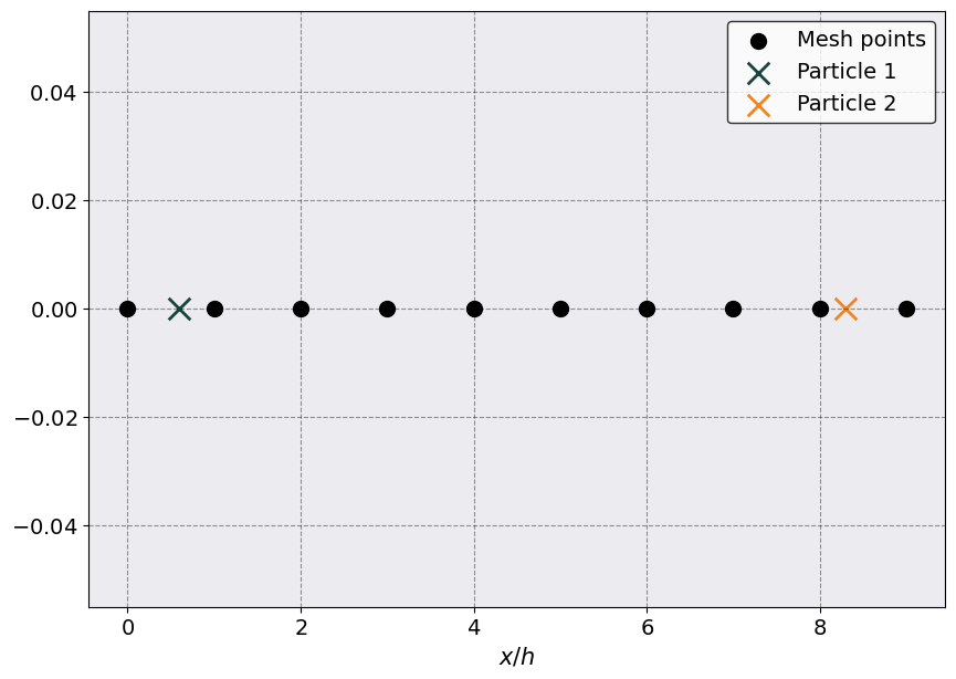
The above plot shows the position of the two particles, represented by X’s, and the location of the mesh points, represented by black dots. Notice that we are rescaling everything by the distance between mesh points, \(h\), which we choose to be = 1 for simplicity.

The next code cell calculates the function \(W(x)\) which represents the amount of charge to be assigned to each mesh point. Particle 1 is distributed over three points while Particle 2 over four mesh points.

[3]:

# Calculate the charge assignment function

# Define the charge assignment order, p
cao1 = 3
cao2 = 4

# Define x_m to be the coordinate of the particle's nearest mesh point (if cao is odd)
x_m1 = rint(x_1/hx - 0.5 *( cao1 % 2 == 0) ).astype(int)
x_m2 = rint(x_2/hx - 0.5 *( cao2 % 2 == 0) ).astype(int)
# The above branchless programming is because int gives the integer value only and not the closest integer

# Distance to the nearest mesh point for p odd
delta_x1 = x_1/hx - x_m1
# Distance to the midpoint between the two nearest mesh points
delta_x2 = x_2/hx - x_m2 - 0.5

# W_3(x_1 - x_m1), W_5(x_2 - x_m2)
# This returns an array of length = p.
# Each element is the fraction of the charge on each of the p mesh points starting from the far left.
wx1 = assgnmnt_func(cao1, delta_x1)
wx2 = assgnmnt_func(cao2, delta_x2)

# Create a long array to plot on the entire x range
full_wx1 = np.zeros( len(x_mesh) )
full_wx2 = np.zeros( len(x_mesh) )

# Note that you need to shift to the left due to zero indexing
ixn = x_m1 - int(cao1/2.0)
# Calculate the W(x) for the first particle
for ix in range(cao1):
    # Check for BC
    if ixn < 0:
        index = ixn + N_mesh_points

    elif ixn > (N_mesh_points -1 ):
        index = ixn - N_mesh_points
    else:
        index = ixn

    full_wx1[index] = wx1[ix]
    ixn += 1

# Note that you need to shift to the left due to zero indexing
ixn = x_m2 - int(cao2/2.0 - 1)
# Calculate the W(x) for the second particle
for ix in range(cao2):
    # Check for BC
    if ixn < 0:
        index = ixn + N_mesh_points
    elif ixn > (N_mesh_points -1 ):
        index = ixn - N_mesh_points
    else:
        index = ixn

    full_wx2[index] = wx2[ix]
    ixn += 1

[4]:

# Make the plot
plt.scatter(x_mesh, np.zeros_like(x_mesh), c = "k", s = 100, label = "Mesh points")
p1 = plt.scatter(x_1, 0, s = 200,  marker = 'x', label = "Particle 1")
plt.scatter(x_m1, 0, s = 200,c = p1.get_facecolor(), marker = 'd', label = "Particle 1 $x_{m1}$")
plt.plot(x_mesh, full_wx1, '--o', c = p1.get_facecolor(), label = r"$W_3(x_1 - x_{m1})$")

p2 = plt.scatter(x_2, 0, s = 200,  marker = 'x', label = "Particle 2")
plt.scatter(x_m2, 0, s = 200,c = p2.get_facecolor(),  marker = 'd', label = "Particle 2 $x_{m2}$")
plt.plot(x_mesh, full_wx2, '--o', c = p2.get_facecolor(), label = r"$W_4(x_2 - x_{m2})$")

plt.legend(ncol = 2)
_ = plt.ylabel(r"$W_p(x)$")
_ = plt.xlabel(r"$x/h$")

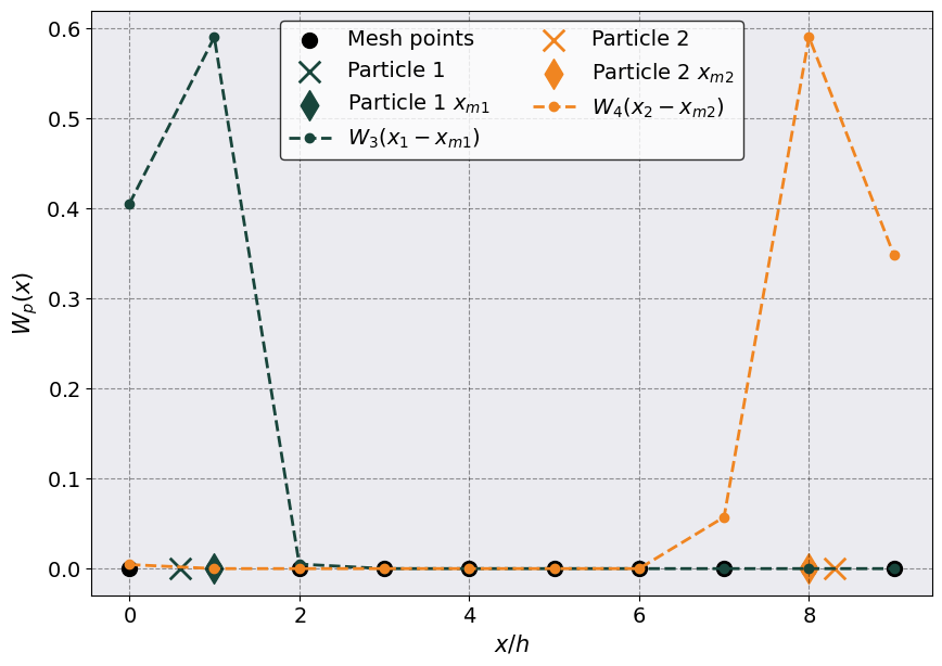
As you can see the first (orange) particle is distributed on the three mesh points (9, 0, 1) while the second (green) particle onto the four mesh points (7, 8, 9, 0).

### 2D Example

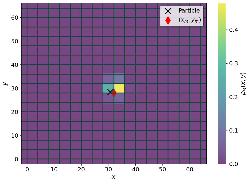
The algorithm described above can be extended to 3D and it is what is contained in the function calc_charge_dens. In the following we will present an example with randomly distributed charges on a 2D plane for visualization.

[5]:

# Calculate the charge assignment function

# Define the charge assignment order, p
cao = 3
x1, y1 = 30.7, 28.3

L = 64
Mx, My = 16, 16
hx, hy = L/Mx, L/My

x_ar = np.linspace(0, L, Mx)
y_ar = np.linspace(0, L, My)
xgrid, ygrid = np.meshgrid(x_ar, y_ar, indexing="ij")

# Define x_m to be the coordinate of the particle's nearest mesh point (if cao is odd)
x_m1 = rint(x1/hx - 0.5 *( cao % 2 == 0) ).astype(int)
y_m1 = rint(y1/hy - 0.5 *( cao % 2 == 0) ).astype(int)
# The above branchless programming is because int gives the integer value only and not the closest integer

# Distance to the nearest mesh point for p odd or midpoint for p even
delta_x = x1/hx - x_m1 - 0.5 *( cao % 2 == 0)
delta_y = y1/hy - y_m1 - 0.5 *( cao % 2 == 0)

# This returns an array of length = p.
# Each element is the fraction of the charge on each of the p mesh points starting from the far left.
wx = assgnmnt_func(cao, delta_x)
wy = assgnmnt_func(cao, delta_y)

# Create a long array to plot on the entire x range
rho_2D = np.zeros_like( xgrid)

# Note that you need to shift to the left due to zero indexing
ixn = x_m1 - int(cao/2.0 - 1  * (cao %2 == 0) )

for ix in range(cao):

    # Check for BC
    index_x = ixn + Mx * (ixn < 0) - Mx*( ixn > (Mx - 1) )

    # Note that you need to shift to the left due to zero indexing
    iyn = y_m1 - int(cao/2.0 -  1 * (cao %2 == 0) )

    for iy in range(cao):
        # Check for BC
        index_y = iyn + My * (iyn < 0) - My*( iyn > (My - 1) )

        rho_2D[index_x, index_y] += wx[ix] * wy[iy]
        iyn += 1
    ixn += 1

[6]:

# I am getting a deprecation warning from matplotlib about the grid in pcolor.
import warnings
warnings.filterwarnings("ignore",category=matplotlib.cbook.mplDeprecation)

fig, ax = plt.subplots(1,1)
p1 = ax.pcolormesh(xgrid, ygrid, rho_2D, alpha = 0.7)
fig.colorbar(p1, label = r"$\rho_M(x,y)$")
ax.scatter(x1, y1, s = 200, marker = "x", c = 'k', label = "Particle")
ax.scatter( (x_m1 )*hx , (y_m1 ) * hy, s = 200, marker = "d", c = 'r', label = "$(x_m, y_m)$")
for i in range(Mx + 1):
    ax.axhline(i * hx)

for j in range(My + 1):
    ax.axvline(j* hy)


ax.legend()
_ = ax.set( xlabel = r"$x$", ylabel = r"$y$")

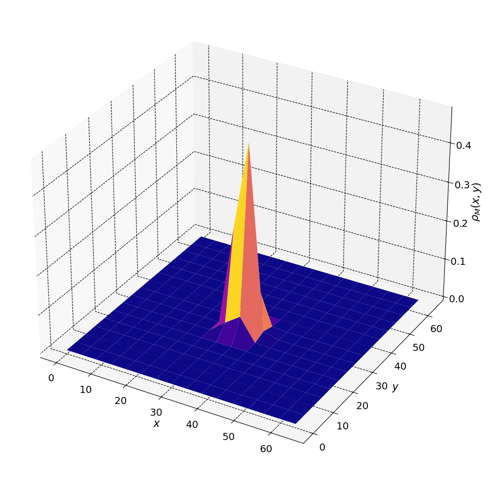
Let’s make the above plot 3D

[7]:

plt.rcParams["axes.facecolor"] = [1, 1, 1]
fig, ax = plt.subplots(figsize=(12, 12),subplot_kw={"projection": "3d"})

ax.plot_surface(xgrid, ygrid, rho_2D, cmap = plt.cm.plasma)
# Uncomment the following if you want to see images of the rho_m duplicated.
# ax.plot_surface(xgrid - L, ygrid, rho_m[0].T, cmap = plt.cm.plasma)
# ax.plot_surface(xgrid - L, ygrid - L, rho_m[0].T, cmap = plt.cm.plasma)
# ax.plot_surface(xgrid , ygrid - L, rho_m[0].T, cmap = plt.cm.plasma)
# ax.plot_surface(xgrid , ygrid + L, rho_m[0].T, cmap = plt.cm.plasma)
# ax.plot_surface(xgrid + L , ygrid + L, rho_m[0].T, cmap = plt.cm.plasma)
# ax.plot_surface(xgrid + L , ygrid, rho_m[0].T, cmap = plt.cm.plasma)
# ax.plot_surface(xgrid + L , ygrid - L, rho_m[0].T, cmap = plt.cm.plasma)
# ax.plot_surface(xgrid - L , ygrid + L, rho_m[0].T, cmap = plt.cm.plasma)
_ = ax.set( xlabel = r"$x$", ylabel = r"$y$", zlabel = r"$\rho_M(x,y)$")

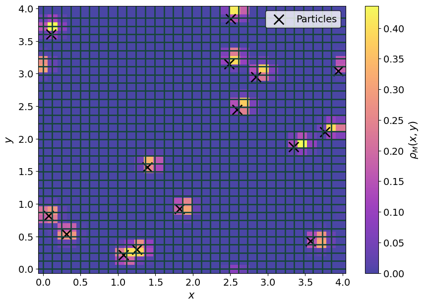
### 2D Example with N particles

Let’s extend the above example to \(N = 15\) particles and use Sarkas’ functions instead.

The function mesh_point_shift calculates the shifts needed if the charge assignment order is even. It returns mid and pshift. mid can be either 0 or 0.5 and it is the equivalent of 0.5 * ( cao % 2 == 0) in the above examples. pshift is the shift in the index, equivalent to int(cao/2 - 1 * (cao%2 == 0)) in the definition of ixn.
The function calc_mesh_coord calculates the mesh coordinates of the particles (mesh_pos) and their corresponding indexes (mesh_points).
The function calc_charge_dens calculates the final charge density rho_m

[8]:

# Number of particles
N = 15
# Box length
L = (4* np.pi * N/3)**(1./3.)
box_lengths = np.ones(3) * L
box_lengths[2] = 0.0

# Charge assignment order
cao = np.array([4, 4, 1])
# Array of mesh points. Note in the case of 2D you still need to pass 1 for the z-mesh
Mx, My = 32, 32
mesh_sz = np.array([Mx, My, 1])
x_ar = np.linspace(0, L, Mx)
y_ar = np.linspace(0, L, My)
xgrid, ygrid = np.meshgrid(x_ar, y_ar, indexing="ij")

# Spacings
h_array = box_lengths/mesh_sz
h_array[2] = 0.0
# print(h_array)

# Particles positions
pos = L * rng.random( size = (N, 3))
pos[:,2] = 0.0 # set the z-coord to 0

charges = np.ones( N, dtype = float)

# Calculate the shifts due to an even cao
mid, pshift = mesh_point_shift(cao)
# Calculates the mesh coordinates of the particles and the corresponding indexes
mesh_pos, mesh_points = calc_mesh_coord(pos, h_array, cao)
# Calculate the total charge density
rho_m = calc_charge_dens(mesh_pos, mesh_points, charges, cao, mesh_sz, mid, pshift)

The first thing to note is the shape of the charge density; it is ( z_mesh, y_mesh, x_mesh). This is a legacy feature that has not been removed.

Let’s plot the charge density

[9]:

fig, ax = plt.subplots(1,1)
p1 = ax.pcolormesh(xgrid, ygrid, rho_m[0].T, cmap = plt.cm.plasma, alpha = 0.75)
fig.colorbar(p1, label = r"$\rho_M(x,y)$")
ax.scatter(pos[:,0], pos[:,1], s = 200, marker = "x", c = 'k', label = "Particles")

for i in range(mesh_sz[0]):
    ax.axhline(i* h_array[0])

for j in range(mesh_sz[1]):
    ax.axvline(j* h_array[1])


ax.legend()
_ = ax.set( xlabel = r"$x$", ylabel = r"$y$")

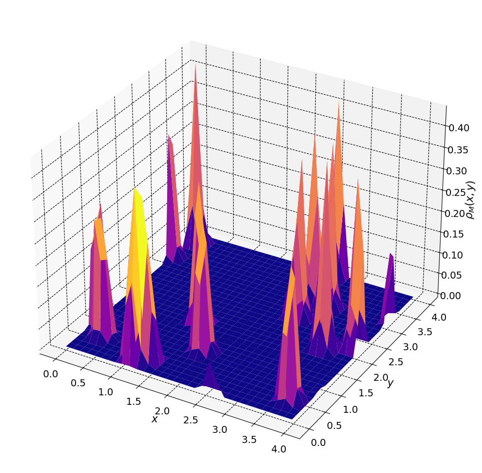
… and its 3D version

[10]:

plt.rcParams["axes.facecolor"] = [1, 1, 1]
fig, ax = plt.subplots(figsize=(12, 12),subplot_kw={"projection": "3d"})

ax.plot_surface(xgrid, ygrid, rho_m[0].T, cmap = plt.cm.plasma)
# Uncomment the following if you want to see images of the rho_m duplicated.
# ax.plot_surface(xgrid - L, ygrid, rho_m[0].T, cmap = plt.cm.plasma)
# ax.plot_surface(xgrid - L, ygrid - L, rho_m[0].T, cmap = plt.cm.plasma)
# ax.plot_surface(xgrid , ygrid - L, rho_m[0].T, cmap = plt.cm.plasma)
# ax.plot_surface(xgrid , ygrid + L, rho_m[0].T, cmap = plt.cm.plasma)
# ax.plot_surface(xgrid + L , ygrid + L, rho_m[0].T, cmap = plt.cm.plasma)
# ax.plot_surface(xgrid + L , ygrid, rho_m[0].T, cmap = plt.cm.plasma)
# ax.plot_surface(xgrid + L , ygrid - L, rho_m[0].T, cmap = plt.cm.plasma)
# ax.plot_surface(xgrid - L , ygrid + L, rho_m[0].T, cmap = plt.cm.plasma)
_ = ax.set( xlabel = r"$x$", ylabel = r"$y$", zlabel = r"$\rho_M(x,y)$")

At this point we need only Fourier transform \(\rho_M(x,y,z)\) and solve Poisson’s equation.

Particle-Particle Particle-Mesh Algorithm

Content