H-He Mixture

In this notebook we will calculate the diffusion and interdiffusion coefficients of Binary Ionic Mixture (BIM) of Hydrogen and Helium. This notebook tries to reproduce the data obtained from Hansen, Joly, and McDonald’s paper.

The YAML input file can be found at input_file and this notebook at notebook.

# Import the usual libraries
%pylab
%matplotlib inline
import os
plt.style.use('MSUstyle')
# Import sarkas
from sarkas.processes import Simulation, PostProcess


# Create the file path to the YAML input file
input_file_name = os.path.join('input_files', 'BIM_cgs.yaml')

Using matplotlib backend: Qt5Agg
Populating the interactive namespace from numpy and matplotlib

Simulation

# sim = Simulation(input_file_name)
# sim.setup(read_yaml=True)
# sim.run()

PostProcessing

postproc = PostProcess(input_file_name)
postproc.setup(read_yaml=True)

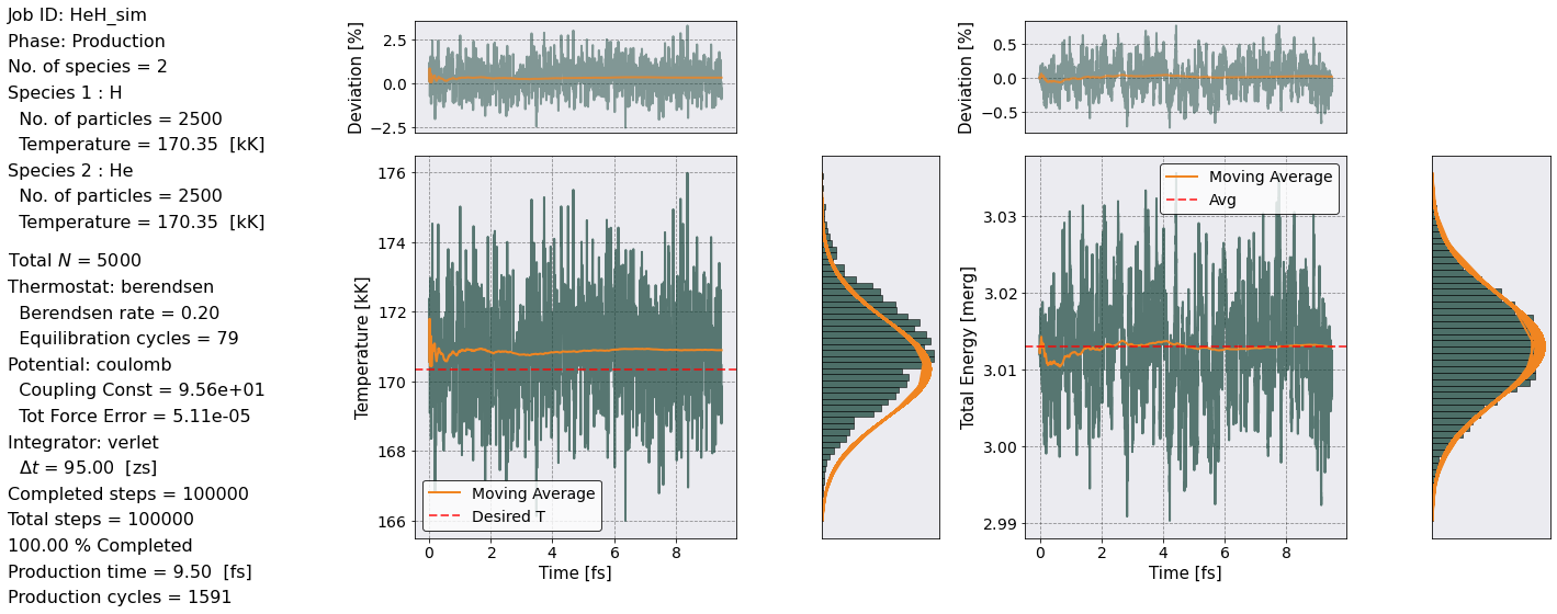
Thermodynamic Check

Let’s make sure that the equilibration phase was \(NVT\) and the production phase \(NVE\).

# Equilibration check
postproc.therm.setup(postproc.parameters)
# postproc.therm.temp_energy_plot(postproc, phase='equilibration')

# Production check
postproc.therm.temp_energy_plot(postproc, phase='production')

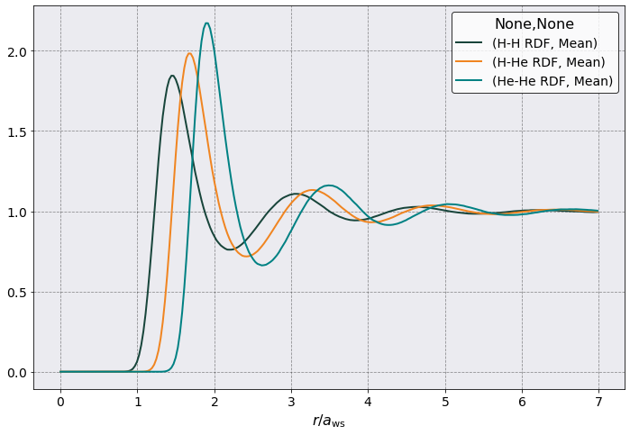
Pair Distribution Function

Let’s look at \(g_{\alpha \beta}(r)\). Just for fun.

postproc.rdf.setup(postproc.parameters)
postproc.rdf.parse()
postproc.rdf.plot(scaling = postproc.parameters.a_ws,
                  y = [("H-H RDF", "Mean"),
                      ("H-He RDF", "Mean"),
                      ("He-He RDF", "Mean")],
                  xlabel = r'$r / a_{\rm ws}$')

<AxesSubplot:xlabel='$r / a_{\\rm ws}$'>

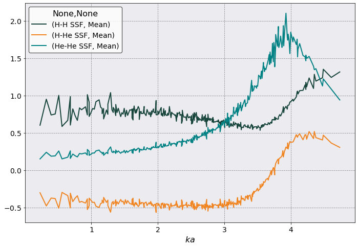
Static Structure Function

Let’s calculate \(S_{\alpha\beta}(k)\) up to \(ka = 5\) and angle average it.

from sarkas.tools.observables import StaticStructureFactor

ssf = StaticStructureFactor()
ssf.no_slices = 4
ssf.angle_averaging = 'full'
ssf.max_ka_value = 5
ssf.setup(postproc.parameters)
ssf.pretty_print()

===================== Static Structure Function ======================

k wavevector information saved in:
 Simulations/HeH_sim/PostProcessing/k_space_data/k_arrays.npz
n(k,t) Data saved in:
 Simulations/HeH_sim/PostProcessing/k_space_data/nkt.h5
Data saved in:
 Simulations/HeH_sim/PostProcessing/StaticStructureFunction/Production/StaticStructureFunction_HeH_sim.h5
Data accessible at: self.k_list, self.k_counts, self.ka_values, self.dataframe

Smallest wavevector k_min = 2 pi / L = 3.9 / N^(1/3)
k_min = 0.2279 / a_ws = 9.2974e+08 [1/cm]

Angle averaging choice: full
        Maximum angle averaged k harmonics = n_x, n_y, n_z = 12, 12, 12
        Largest angle averaged k_max = k_min * sqrt( n_x^2 + n_y^2 + n_z^2)
        k_max = 4.7377 / a_ws = 1.9324e+10 [1/cm]

Total number of k values to calculate = 2196
No. of unique ka values to calculate = 354

ssf.parse()
ssf.dataframe

	Inverse Wavelength	H-H SSF		H-He SSF		He-He SSF
	NaN	Mean	Std	Mean	Std	Mean	Std
0	9.297400e+08	0.602529	0.602529	-0.301900	-0.301900	0.151476	0.151476
1	1.314851e+09	0.950866	0.950866	-0.477511	-0.477511	0.240235	0.240235
2	1.610357e+09	0.739990	0.739990	-0.372485	-0.372485	0.188129	0.188129
3	1.859480e+09	0.752397	0.752397	-0.379395	-0.379395	0.192214	0.192214
4	2.078962e+09	1.002572	1.002572	-0.506872	-0.506872	0.257413	0.257413
...	...	...	...	...	...	...	...
349	1.785972e+10	1.192680	1.192680	0.436384	0.436384	1.359468	1.359468
350	1.826649e+10	1.237796	1.237796	0.405055	0.405055	1.127594	1.127594
351	1.831376e+10	1.351196	1.351196	0.469020	0.469020	1.221888	1.221888
352	1.880283e+10	1.242406	1.242406	0.364108	0.364108	1.086201	1.086201
353	1.932428e+10	1.315648	1.315648	0.305602	0.305602	0.940871	0.940871

354 rows × 7 columns

ssf.plot(
    scaling = 1 /ssf.a_ws,
    y= [('H-H SSF', 'Mean'), ('H-He SSF', 'Mean'), ('He-He SSF', 'Mean')],
    xlabel = r'$ka$')

<AxesSubplot:xlabel='$ka$'>

Interdiffusion

The interdiffusion coefficient is calculated by the Green-Kubo relation

\[D_{12} = \frac{\mathcal{J}}{3Nx_1x_2} \int_0^\infty dt {\rm{{ACF}_{ID}}} = \frac{\mathcal{J}}{3Nx_1x_2} \int_0^\infty dt \langle \mathbf{j}(0) \cdot \mathbf{j}(t) \rangle,\]

where \(\mathcal{J}\) is the thermodynamic factor

\[\mathcal{J} = \frac{x_1x_2}{S_{cc}(k = 0)}\]

and \(S_{cc}(k)\) is the concentration-concentration structure factor that can be decomposed into partial structure factors as

\[S_{cc}(k) = x_1x_2[x_2S_{11}(k) + x_1S_{22}(k) - 2\sqrt{x_1x_2}S_{12}(k)].\]

Calculating the interdiffusion coefficient \(D_{12}\) is two-fold in that we must compute the auto-correlation function \(\rm{{ACF}_{ID}}\) and the thermodynamic factor \(\mathcal J\).

We will calculate \(\mathcal J\) first by fitting the following function to \(S_{\alpha\beta}(k)\)

# Define fitting functions
from scipy.optimize import curve_fit

def poly_fit(x, a, b, c):
    return a*x**2 + b*x + c

def lin_fit(x, a, b):
    return a*x + b

def inv_fit(x, a, b, c):
    return a*np.exp(b*x) + c

As you can see from above \(S_{\alpha\beta}(k)\) are pretty noisy. Therefore we choose only those \(ka\) values for which we have averaged more than three \(S_{\alpha\beta}(k)\).

# Create masks
mask = ssf.k_counts > 3
ka_values_full = ssf.ka_values[mask]

ka_mask = ka_values_full < 3.0
ka_values = ka_values_full[ka_mask]

# Remake the plot
fig, ax = plt.subplots(1,1, figsize = (12,9))
ssf.plot(
    scaling = 1 /ssf.a_ws,
    y= [('H-H SSF', 'Mean'), ('H-He SSF', 'Mean'), ('He-He SSF', 'Mean')],
    xlabel = r'$ka$', ax = ax)

# H-H Fit and plot
sk_array_full = ssf.dataframe[("H-H SSF", 'Mean')].to_numpy()
sk_array = sk_array_full[mask]
poptH, pcov = curve_fit(poly_fit, ka_values, sk_array[ka_mask])
ax.plot(ka_values, poly_fit(ka_values, *poptH), ls='--', label = 'Fit H-H')

# H-He Fit and plot
sk_array_full = ssf.dataframe[("H-He SSF", 'Mean')].to_numpy()
sk_array = sk_array_full[mask]
poptHHe, pcov = curve_fit(lin_fit, ka_values, sk_array[ka_mask])
ax.plot(ka_values, lin_fit(ka_values, *poptHHe),  ls='--', label = 'Fit H-He')

# He-He Fit and plot
sk_array_full = ssf.dataframe[("He-He SSF", 'Mean')].to_numpy()
sk_array = sk_array_full[mask]
poptHe, pcov = curve_fit(inv_fit, ka_values, sk_array[ka_mask])
ax.plot(ka_values, inv_fit(ka_values, *poptHe),  ls='--', label = 'Fit He-He')

ax.legend(ncol =2 )

<matplotlib.legend.Legend at 0x7f40cc244550>

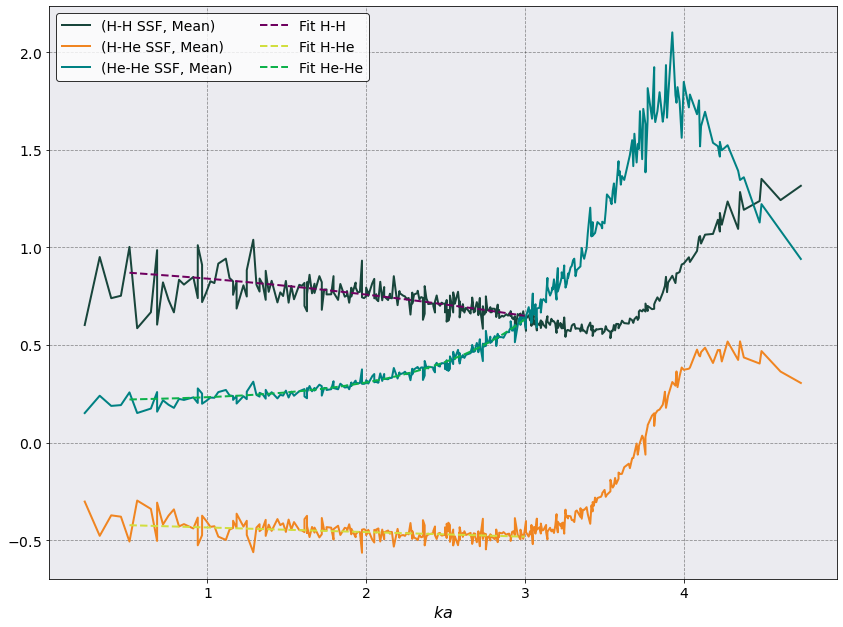
Pretty good, right? Now for the thermodynamic factor

x1, x2 = ssf.species_concentrations
Scc_k0 = x1*x2*(x2*inv_fit(0, *poptHe) + x1*poly_fit(0, *poptH) - 2*np.sqrt(x1*x2)*lin_fit(0, *poptHHe))
Therm_factor = x1*x2/Scc_k0
print('J = {:.4f}'.format(Therm_factor) )

J = 1.0354

The value is ~ 1 which is what Hansen et al. assumed. Therefore we won’t use it below.

Transport Coefficients in Sarkas

Calculating transport coefficients is easy once the TransportCoefficients class from the sarkas.tools.transport subpackage is imported.

Interdiffusion is a method of TransportCoefficients as such we need to initialize the class first which requires the following inputs

Parameters
----------
params : sarkas.base.Parameters
    Simulation's parameters.

phase : str, optional
    Phase to compute. Default = 'production'.

no_slices : int, optional
    Number of slices of the simulation. Default = 1.

**kwargs:
    Arguments to pass :meth:`sarkas.tools.observables.FluxAutoCorrelationFunction`

The parameter params is required as it contains relevant information. Notice the parameter no_slices. This represents the number of divisions in which we want to divide the full length of the time series. For each of these slices the method will integrate the ACF of the observable to get the transport coefficient.

The calculation of the transport coefficient is achieved by calling the method and passing the appropriate observable objects. The docstring can be found here. As you can see it requires the appropriate observable which in this case is interdiffusion_df_slices. The transport coefficient of each slice will be stored as a column of a pandas.DataFrame called interdiffusion_df_slices, the Mean and Std (over slices) will be stored in the interdiffusion_df.

The first column of these dataframes corresponds to the time in sec of each timestep.

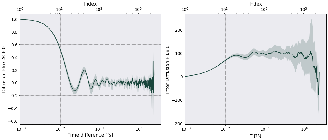
The option plot=True will make a figure with two plots. On the left the ACF as a function of time and on the right a plot of the transport coefficient as a function of time with the corresponding errorband.

from sarkas.tools.transport import TransportCoefficients
from sarkas.tools.observables import DiffusionFlux

# Compute the diffusion flux by dividing the simulations into 4 smaller simulations
jc_acf = DiffusionFlux()
jc_acf.no_slices = 4
jc_acf.setup(postproc.parameters)
jc_acf.parse()

# Let's look at it
jc_acf.dataframe_slices

	Time	Diffusion Flux 0
	NaN	X	Y	Z	X	Y	Z	X	Y	Z	X	Y	Z
	NaN	slice 0	slice 0	slice 0	slice 1	slice 1	slice 1	slice 2	slice 2	slice 2	slice 3	slice 3	slice 3
0	0.000000e+00	1.993921e-31	-8.374467e-31	-9.471123e-32	1.650410e-16	-2.750060e-16	-2.132580e-17	-2.592813e-16	-4.231939e-16	5.125572e-16	-4.154773e-17	3.628596e-16	2.464266e-16
1	9.500000e-19	3.019202e-17	2.536946e-17	3.126571e-18	1.526589e-16	-2.982007e-16	-4.579669e-17	-2.251972e-16	-4.231959e-16	5.181452e-16	-5.253896e-17	3.379070e-16	2.268565e-16
2	1.900000e-18	6.201764e-17	4.934061e-17	4.431807e-18	1.391056e-16	-3.185411e-16	-6.691581e-17	-1.916298e-16	-4.200004e-16	5.135595e-16	-6.553873e-17	3.107889e-16	2.084986e-16
3	2.850000e-18	9.485616e-17	7.177066e-17	3.852522e-18	1.244862e-16	-3.358978e-16	-8.393863e-17	-1.592913e-16	-4.137426e-16	4.986987e-16	-8.010234e-17	2.817022e-16	1.911914e-16
4	3.800000e-18	1.280001e-16	9.259796e-17	1.410964e-18	1.089811e-16	-3.501835e-16	-9.631634e-17	-1.288192e-16	-4.046605e-16	4.736470e-16	-9.582756e-17	2.509364e-16	1.746648e-16
...	...	...	...	...	...	...	...	...	...	...	...	...	...
2495	2.370250e-15	2.099584e-16	-1.233453e-16	1.169715e-16	-4.095864e-16	-3.794951e-16	3.462978e-16	-3.117694e-17	4.556562e-16	3.596185e-16	-7.628444e-16	4.937378e-16	-1.258954e-16
2496	2.371200e-15	2.029564e-16	-1.575947e-16	9.064110e-17	-3.848219e-16	-3.929576e-16	3.959465e-16	-2.623574e-17	4.408110e-16	3.357565e-16	-7.430279e-16	4.567765e-16	-1.791263e-16
2497	2.372150e-15	1.950846e-16	-1.901676e-16	6.264069e-17	-3.566792e-16	-4.045290e-16	4.381401e-16	-2.503433e-17	4.243542e-16	3.121659e-16	-7.191573e-16	4.188821e-16	-2.290961e-16
2498	2.373100e-15	1.862069e-16	-2.207674e-16	3.393836e-17	-3.258457e-16	-4.136707e-16	4.720722e-16	-2.739204e-17	4.060086e-16	2.892282e-16	-6.922675e-16	3.801472e-16	-2.746724e-16
2499	2.374050e-15	1.762159e-16	-2.491263e-16	5.591958e-18	-2.931044e-16	-4.199792e-16	4.970616e-16	-3.302129e-17	3.855537e-16	2.672468e-16	-6.633041e-16	3.405559e-16	-3.149317e-16

2500 rows × 13 columns

Notice that there is a column Diffusion Flux 0 and Diffusion Flux ACF 0 for each slice. For the transport coefficient I will use Diffusion Flux ACF 0.

tc = TransportCoefficients(
        postproc.parameters,
        no_slices = 4)
tc.interdiffusion(jc_acf, plot = True)
# Note the info printed to screen

===================== Interdiffusion Coefficient =====================

Data saved in:
 Simulations/HeH_sim/PostProcessing/TransportCoefficients/Production/Interdiffusion_HeH_sim.h5
Simulations/HeH_sim/PostProcessing/TransportCoefficients/Production/Interdiffusion_slices_HeH_sim.h5

No. of slices = 4
No. dumps per slice = 250
Time interval of autocorrelation function = 2.3750e-15 [s] ~ 397 w_p T

# Let's look at what we have
tc.interdiffusion_df

	Time	Inter Diffusion Flux 0
	NaN	Mean	Std
0	0.000000e+00	0.000000	0.000000e+00
1	9.500000e-19	0.000000	0.000000e+00
2	1.900000e-18	0.000008	3.826732e-07
3	2.850000e-18	0.000017	7.656943e-07
4	3.800000e-18	0.000025	1.148443e-06
...	...	...	...
2495	2.370250e-15	0.000012	1.937744e-04
2496	2.371200e-15	0.000014	1.957540e-04
2497	2.372150e-15	0.000016	1.975726e-04
2498	2.373100e-15	0.000017	1.992226e-04
2499	2.374050e-15	0.000018	2.006965e-04

2500 rows × 3 columns

As mentioned the InterDiffusion is calculated for each slice and then averaged. The left plot above shows the mean over the four slices of the Diffusion Flux ACF with its standard deviation as the shaded area. The upper x-axis (Index) indicates the index value in the dataframe.

Let’s now plot this and compare with Hansen et al. result.

aws = postproc.parameters.a_ws
vaa = postproc.parameters.hydrodynamic_frequency
norm = 1/(vaa * aws**2 )

fig, ax = plt.subplots(1,1)
ax.plot(
    tc.interdiffusion_df["Time"]*1e15,
    tc.interdiffusion_df[("Inter Diffusion Flux 0","Mean")] * norm ,
    label = 'Sarkas')
ax.plot(
    tc.interdiffusion_df["Time"]*1e15,
    norm * tc.interdiffusion_df[("Inter Diffusion Flux 0","Mean")].expanding().mean())

ax.fill_between(
    tc.interdiffusion_df["Time"].iloc[:,0]*1e15, # I don't understand why I need iloc here but not above
    (tc.interdiffusion_df[("Inter Diffusion Flux 0","Mean")] - tc.interdiffusion_df[("Inter Diffusion Flux 0","Std")])*norm,
    (tc.interdiffusion_df[("Inter Diffusion Flux 0","Mean")] + tc.interdiffusion_df[("Inter Diffusion Flux 0","Std")])*norm,
    alpha = 0.4)

ax.axhline(0.0109, color = 'r', ls = '--', label='HJM value')
ax.legend()
ax.set(xscale = 'log', xlabel = 'Time [fs]', title = r'H-He Interdiffusion $\Gamma = 40$')

[None,
 Text(0.5, 0, 'Time [fs]'),
 Text(0.5, 1.0, 'H-He Interdiffusion $\\Gamma = 40$')]

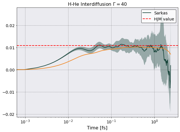
Looks good to me!