Quickstart#

Once installation is complete you can start running Sarkas. This quickstart guide will walk you through a simple example in order to check that everything is running smoothly.

The YAML input file can be found at input_file and this notebook at notebook

Simulation#

In Jupyter notebook you can run the following commands

[1]:

# Import the usual libraries
%pylab
%matplotlib inline
import os

plt.style.use('MSUstyle')

# Import sarkas
from sarkas.processes import Simulation, PostProcess

# Create the file path to the YAML input file
input_file_name = os.path.join('input_files', 'yocp_quickstart.yaml')

Using matplotlib backend: Qt5Agg
Populating the interactive namespace from numpy and matplotlib

The above commands imported the required libraries and define the file path to our input file.

Let’s now run the simulation

[2]:

# Initialize the Simulation class
sim = Simulation(input_file_name)
# Setup the simulation's parameters
sim.setup(read_yaml=True)
# Run the simulation
sim.run()






 _______              __
|     __|.---.-.----.|  |--.---.-.-----.
|__     ||  _  |   _||    <|  _  |__ --|
|_______||___._|__|  |__|__|___._|_____|



An open-source pure-python molecular dynamics suite for non-ideal plasmas.





* * * * * * * * * * * * * * * * * * * * * * * * * * * * * * * * * * * * * * * * * * * * * * * * * *
                                   Simulation
* * * * * * * * * * * * * * * * * * * * * * * * * * * * * * * * * * * * * * * * * * * * * * * * * *

Job ID:  yocp_quickstart
Job directory:  Simulations/yocp_quickstart

Equilibration dumps directory:
 Simulations/yocp_quickstart/Simulation/Equilibration/dumps
Production dumps directory:
 Simulations/yocp_quickstart/Simulation/Production/dumps

Equilibration Thermodynamics file:
 Simulations/yocp_quickstart/Simulation/Equilibration/EquilibrationEnergy_yocp_quickstart.csv
Production Thermodynamics file:
 Simulations/yocp_quickstart/Simulation/Production/ProductionEnergy_yocp_quickstart.csv

PARTICLES:
Total No. of particles =  1000
No. of species =  1
Species ID: 0
        Name: C
        No. of particles = 1000
        Number density = 1.136669e+23 [N/cc]
        Atomic weight = 12.0105 [a.u.]
        Mass = 2.008900e-23 [g]
        Mass density = 2.283455e+00 [g/cc]
        Charge number/ionization degree = 1.9766
        Charge = 9.494010e-10 [esu]
        Temperature = 5.000000e+03 [K] = 4.308667e-01 [eV]
        Debye Length = 7.322426e-10 [1/cm^3]
        Plasma Frequency = 2.531585e+14 [rad/s]

SIMULATION AND INITIAL PARTICLE BOX:
Units:  cgs
Wigner-Seitz radius = 1.280636e-08 [cm]
No. of non-zero box dimensions =  3
Box side along x axis = 1.611992e+01 a_ws = 2.064375e-07 [cm]
Box side along y axis = 1.611992e+01 a_ws = 2.064375e-07 [cm]
Box side along z axis = 1.611992e+01 a_ws = 2.064375e-07 [cm]
Box Volume = 8.797633e-21 [cm^3]
Initial particle box side along x axis = 1.611992e+01 a_ws = 2.064375e-07 [cm]
Initial particle box side along y axis = 1.611992e+01 a_ws = 2.064375e-07 [cm]
Initial particle box side along z axis = 1.611992e+01 a_ws = 2.064375e-07 [cm]
Initial particle box Volume = 8.797633e-21 [cm^3]
Boundary conditions: periodic

ELECTRON PROPERTIES:
Number density: n_e = 2.246739e+23 [N/cc]
Wigner-Seitz radius: a_e = 1.020437e-08 [cm]
Temperature: T_e = 5.000000e+03 [K] = 4.308667e-01 [eV]
de Broglie wavelength: lambda_deB = 1.054132e-07 [cm]
Thomas-Fermi length: lambda_TF = 4.702909e-09 [cm]
Fermi wave number: k_F = 1.880722e+08 [1/cm]
Fermi Energy: E_F = 1.347634e+01 [eV]
Relativistic parameter: x_F = 7.262582e-03 --> E_F = 1.347617e+01 [eV]
Degeneracy parameter: Theta = 3.197207e-02
Coupling: r_s = 1.928347,  Gamma_e = 32.750858
Warm Dense Matter Parameter: W = 3.8973e-03
Chemical potential: mu = 3.1251e+01 k_B T_e = 9.9916e-01 E_F

POTENTIAL:  yukawa
electron temperature = 5.0000e+03 [K] = 4.3087e-01 [eV]
kappa = 2.7231
Gamma_eff = 101.96

ALGORITHM:  pp
rcut = 4.6852 a_ws = 6.000000e-08 [cm]
No. of PP cells per dimension =  3,  3,  3
No. of particles in PP loop =    662
No. of PP neighbors per particle =    102
Tot Force Error = 5.818612e-06

THERMOSTAT:
Type: berendsen
First thermostating timestep, i.e. relaxation_timestep = 300
Berendsen parameter tau: 2.000 [timesteps]
Berendsen relaxation rate: 0.500 [1/timesteps]
Thermostating temperatures:
Species ID 0: T_eq = 5.000000e+03 [K] = 4.308667e-01 [eV]

INTEGRATOR:
Type: verlet
Time step = 5.000000e-17 [s]
Total plasma frequency = 2.531585e+14 [rad/s]
w_p dt = 0.0127 ~ 1/79

Equilibration:
No. of equilibration steps = 10000
Total equilibration time = 5.0000e-13 [s] ~ 126 w_p T_eq
snapshot interval step = 10
snapshot interval time = 5.0000e-16 [s] = 0.1266 w_p T_snap
Total number of snapshots = 1000

Production:
No. of production steps = 20000
Total production time = 1.0000e-12 [s] ~ 253 w_p T_prod
snapshot interval step = 10
snapshot interval time = 5.0000e-16 [s] = 0.1266 w_p T_snap
Total number of snapshots = 2000


------------------------ Initialization Times ------------------------


Potential Initialization Time: 1 sec 95 msec 165 usec 515 nsec

Particles Initialization Time: 0 sec 0 msec 354 usec 373 nsec

Total Simulation Initialization Time: 1 sec 95 msec 165 usec 515 nsec


--------------------------- Equilibration ----------------------------


Equilibration Time: 0 hrs 1 min 35 sec


----------------------------- Production -----------------------------


Production Time: 0 hrs 3 min 30 sec

Total Time: 0 hrs 5 min 6 sec

Postprocessing#

Now that our simulation is complete we need to check if the simulation was physically sound. Run the following three lines will initialize the PostProcess class and calculate the observables defined in the input file.

It will also produce a plot of the Temperature and Total Energy of the Production phase.

[3]:

# Initialize the Postprocessing class
postproc = PostProcess(input_file_name)
# Read the simulation's parameters and assign attributes
postproc.setup(read_yaml=True)
# Calculate observables
postproc.run()




* * * * * * * * * * * * * * * * * * * * * * * * * * * * * * * * * * * * * * * * * * * * * * * * * *
                                 Postprocessing
* * * * * * * * * * * * * * * * * * * * * * * * * * * * * * * * * * * * * * * * * * * * * * * * * *

Job ID:  yocp_quickstart
Job directory:  Simulations/yocp_quickstart
PostProcessing directory:
 Simulations/yocp_quickstart/PostProcessing

Equilibration dumps directory:  Simulations/yocp_quickstart/Simulation/Equilibration/dumps
Production dumps directory:
 Simulations/yocp_quickstart/Simulation/Production/dumps

Equilibration Thermodynamics file:
 Simulations/yocp_quickstart/Simulation/Equilibration/EquilibrationEnergy_yocp_quickstart.csv
Production Thermodynamics file:
 Simulations/yocp_quickstart/Simulation/Production/ProductionEnergy_yocp_quickstart.csv


==================== Radial Distribution Function ====================

Data saved in:
 Simulations/yocp_quickstart/PostProcessing/RadialDistributionFunction/Production/RadialDistributionFunction_yocp_quickstart.h5
Data accessible at: self.ra_values, self.dataframe

No. bins = 250
dr = 0.0187 a_ws = 2.4000e-10 [cm]
Maximum Distance (i.e. potential.rc)= 4.6852 a_ws = 6.0000e-08 [cm]


Radial Distribution Function Calculation Time: 0 sec 62 msec 472 usec 771 nsec

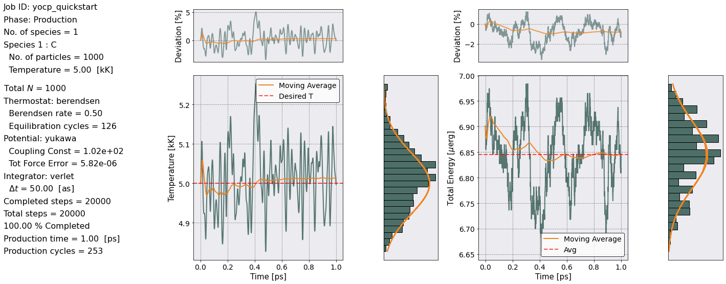
../../_images/documentation_Tutorial_NB_Quickstart_5_3.png

You will notice that both the energy and temperature oscillates wildly. This is fine as long as the percentage deviations, in the top plots, are small. You should have a temperature deviations between -2% to ~ 4-5% while energy deviations between -2% and 1%.

Observables#

The most common observable is the radial distribution function. This was calculated by postproc.run(), here we plot it by rescaling the x axis by the Wigner-Seitz radius \(a_{\rm ws}\).

[4]:

# Initialize the Pair Distribution Function class
ax = postproc.rdf.plot(
    scaling=postproc.parameters.a_ws,
    y = [("C-C RDF", "Mean")],
    xlabel = r'$r/a_{\rm ws}$',
    ylabel = r'$g(r)$'
)
ax.legend(["C-C RDF"])

[4]:

<matplotlib.legend.Legend at 0x7f43925b7690>

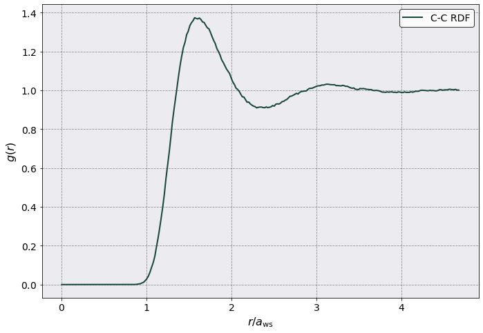
../../_images/documentation_Tutorial_NB_Quickstart_7_1.png

Things to check in here are:

Does \(g(r)\) go to 1 for large \(r\) values ?
Is there a peak at \(r \sim ~1.5 a\) ?
Is the height of this peak about ~ 1.4?

If the answer to all these question is yes than the simulation was successfull.

Quickstart

Content

Quickstart#

Simulation#

Postprocessing#

Observables#