Magnetized Plasma

This codes tests the Boris magnetic integrator by reproducing results of Bernu Journal de Physique, 42 L253 (1981).

We simulate a One Component Plasma composed of \(N = 1000\) Hydrogen atoms at a density of \(n = 1.62 \times 10^{30}\) \(N/m^3\), and temperature \(T = 0.3\) \(eV\), which leads to \(\Gamma = 100\). The system is in a constant magnetic field \(B = B_0 \hat{\mathbf z}\) with \(B_0 = 17 \times 10^6\) Tesla. The ratio of the cyclotron frequency to the plasma frequency is \(\beta \sim 1.0\).

The YAML input file can be found at input_file and this notebook at notebook.

# Import the usual libraries
%pylab
%matplotlib inline
import os

plt.style.use('MSUstyle')
# Import sarkas
from sarkas.processes import Simulation, PostProcess, PreProcess

# Create the file path to the YAML input file
input_file_name = os.path.join('input_files',  'mag_ocp_mks_boris.yaml')

Using matplotlib backend: Qt5Agg
Populating the interactive namespace from numpy and matplotlib

Preprocessing

preproc = PreProcess(input_file_name)
preproc.setup(read_yaml=True)
preproc.run(timing=True, loops=100, pppm_estimate = True)

  _________             __
 /   _____/____ _______|  | _______    ______
 \_____  \\__  \\_  __ \  |/ /\__  \  /  ___/
 /        \/ __ \|  | \/    <  / __ \_\___ \
/_______  (____  /__|  |__|_ \(____  /____  >
        \/     \/           \/     \/     \/


An open-source pure-python molecular dynamics suite for non-ideal plasmas.





* * * * * * * * * * * * * * * * * * * * * * * * * * * * * * * * * * * * * * * * * * * * * * * * * *
                                 Preprocessing
* * * * * * * * * * * * * * * * * * * * * * * * * * * * * * * * * * * * * * * * * * * * * * * * * *

Job ID:  ocp_mag_boris
Job directory:  Simulations/ocp_mag_boris

Equilibration dumps directory:
 Simulations/ocp_mag_boris/PreProcessing/Equilibration/dumps
Production dumps directory:
 Simulations/ocp_mag_boris/PreProcessing/Production/dumps

Equilibration Thermodynamics file:
 Simulations/ocp_mag_boris/PreProcessing/Equilibration/EquilibrationEnergy_ocp_mag_boris.csv
Production Thermodynamics file:
 Simulations/ocp_mag_boris/PreProcessing/Production/ProductionEnergy_ocp_mag_boris.csv

PARTICLES:
Total No. of particles =  1000
No. of species =  1
Species ID: 0
        Name: H
        No. of particles = 1000
        Number density = 1.620000e+30 [N/m^3]
        Atomic weight = 1.0002 [a.u.]
        Mass = 1.673000e-27 [kg]
        Mass density = 2.710260e+03 [kg/m^3]
        Charge number/ionization degree = 1.0000
        Charge = 1.602177e-19 [C]
        Temperature = 3.330091e+03 [K] = 2.869650e-01 [eV]
        Debye Length = 3.128788e-12 [1/m]
        Plasma Frequency = 1.675504e+15 [rad/s]
        Cyclotron Frequency = 1.628034e+15 [rad/s]
        beta_c = 0.9717

SIMULATION AND INITIAL PARTICLE BOX:
Units:  mks
Wigner-Seitz radius = 5.282005e-11 [m]
No. of non-zero box dimensions =  3
Box side along x axis = 1.611992e+01 a_ws = 8.514549e-10 [m]
Box side along y axis = 1.611992e+01 a_ws = 8.514549e-10 [m]
Box side along z axis = 1.611992e+01 a_ws = 8.514549e-10 [m]
Box Volume = 6.172840e-28 [m^3]
Initial particle box side along x axis = 1.611992e+01 a_ws = 8.514549e-10 [m]
Initial particle box side along y axis = 1.611992e+01 a_ws = 8.514549e-10 [m]
Initial particle box side along z axis = 1.611992e+01 a_ws = 8.514549e-10 [m]
Initial particle box Volume = 6.172840e-28 [m^3]
Boundary conditions: periodic

ELECTRON PROPERTIES:
Number density: n_e = 1.620000e+30 [N/m^3]
Wigner-Seitz radius: a_e = 5.282005e-11 [m]
Temperature: T_e = 3.330091e+03 [K] = 2.869650e-01 [eV]
de Broglie wavelength: lambda_deB = 1.291671e-09 [m]
Thomas-Fermi length: lambda_TF = 3.382169e-11 [m]
Fermi wave number: k_F = 3.633390e+10 [1/m]
Fermi Energy: E_F = 5.029756e+01 [eV]
Relativistic parameter: x_F = 1.403067e-02 --> E_F = 5.029509e+01 [eV]
Degeneracy parameter: Theta = 5.705346e-03
Coupling: r_s = 0.998154,  Gamma_e = 95.000103
Warm Dense Matter Parameter: W = 2.4019e-04
Chemical potential: mu = 1.7527e+02 k_B T_e = 9.9997e-01 E_F
Electron cyclotron frequency: w_c = 2.989994e+18
Lowest Landau energy level: h w_c/2 = 1.576582e-16
Electron magnetic energy gap: h w_c = 3.153163e-16 = 3.9128e+01 E_F = 6.8582e+03 k_B T_e

MAGNETIC FIELD:
Magnetic Field = [0.0000e+00, 0.0000e+00, 1.7000e+07] [Tesla]
Magnetic Field Magnitude = 1.7000e+07 [Tesla]
Magnetic Field Unit Vector = [0.0000e+00, 0.0000e+00, 1.0000e+00]

POTENTIAL:  coulomb
Effective Coupling constant: Gamma_eff = 95.00
Short-range Cutoff radius: rs = 0.000000e+00 [m]

ALGORITHM:  pppm
Charge assignment order: 6
FFT aliases: [3, 3, 3]
Mesh: 64 x 64 x 64
Ewald parameter alpha = 0.9000 / a_ws = 1.703898e+10 [1/m]
Mesh width = 0.2519, 0.2519, 0.2519 a_ws
           = 1.3304e-11, 1.3304e-11, 1.3304e-11 [m]
Mesh size * Ewald_parameter (h * alpha) = 0.2267, 0.2267, 0.2267
                                        ~ 1/4, 1/4, 1/4
rcut = 4.1700 a_ws = 2.202596e-10 [m]
No. of PP cells per dimension =  3,  3,  3
No. of particles in PP loop =    467
No. of PP neighbors per particle =     72
PM Force Error = 5.073538e-07
PP Force Error = 3.654934e-07
Tot Force Error = 6.252946e-07

THERMOSTAT:
Type: berendsen
First thermostating timestep, i.e. relaxation_timestep = 100
Berendsen parameter tau: 10.000 [timesteps]
Berendsen relaxation rate: 0.100 [1/timesteps]
Thermostating temperatures:
Species ID 0: T_eq = 3.330091e+03 [K] = 2.869650e-01 [eV]

INTEGRATOR:
Type: magnetic_boris_zdir
Time step = 1.100000e-17 [s]
Total plasma frequency = 1.675504e+15 [rad/s]
w_p dt = 0.0184 ~ 1/54

Equilibration:
No. of equilibration steps = 5000
Total equilibration time = 5.5000e-14 [s] ~ 92 w_p T_eq
snapshot interval step = 10
snapshot interval time = 1.1000e-16 [s] = 0.1843 w_p T_snap
Total number of snapshots = 500
Electrostatic Equilibration Type: magnetic_boris

Magnetization:
No. of magnetization steps = 5000
Total magnetization time = 5.5000e-14 [s] ~ 92 w_p T_mag
snapshot interval step = 10
snapshot interval time = 1.1000e-16 [s] = 0.1843 w_p T_snap
Total number of snapshots = 500

Production:
No. of production steps = 70000
Total production time = 7.7000e-13 [s] ~ 1290 w_p T_prod
snapshot interval step = 5
snapshot interval time = 5.5000e-17 [s] = 0.0922 w_p T_snap
Total number of snapshots = 14000


------------------------ Initialization Times ------------------------


Potential Initialization Time: 0 hrs 0 min 5 sec

Particles Initialization Time: 0 sec 0 msec 448 usec 27 nsec

Total Simulation Initialization Time: 0 hrs 0 min 5 sec


========================== Times Estimates ===========================

Optimal Green's Function Time:
0 min 3 sec 581 msec 556 usec 188 nsec

Time of PP acceleration calculation averaged over 100 steps:
0 min 0 sec 6 msec 205 usec 565 nsec

Time of PM acceleration calculation averaged over 100 steps:
0 min 0 sec 31 msec 773 usec 550 nsec


Running 101 equilibration and production steps to estimate simulation times

Time of a single equilibration step averaged over 100 steps:
0 min 0 sec 42 msec 600 usec 652 nsec

Time of a single magnetization step averaged over 100 steps:
0 min 0 sec 38 msec 760 usec 2 nsec

Time of a single production step averaged over 100 steps:
0 min 0 sec 39 msec 127 usec 955 nsec



----------------------- Total Estimated Times ------------------------


Equilibration Time: 0 hrs 3 min 33 sec

Magnetization Time: 0 hrs 3 min 13 sec

Production Time: 0 hrs 45 min 38 sec

Total Run Time: 0 hrs 52 min 25 sec


========================= Filesize Estimates =========================


Equilibration:

Checkpoint filesize: 0 GB 0 MB 154 KB 10 bytes
Checkpoint folder size: 0 GB 75 MB 204 KB 904 bytes

Magnetization:

Checkpoint filesize: 0 GB 0 MB 154 KB 10 bytes
Checkpoint folder size: 0 GB 75 MB 204 KB 904 bytes

Production:

Checkpoint filesize: 0 GB 0 MB 154 KB 10 bytes
Checkpoint folder size: 2 GB 57 MB 616 KB 736 bytes

Total minimum needed space: 2 GB 208 MB 2 KB 496 bytes

Figures can be found in Simulations/ocp_mag_boris/PreProcessing/PPPM_Plots

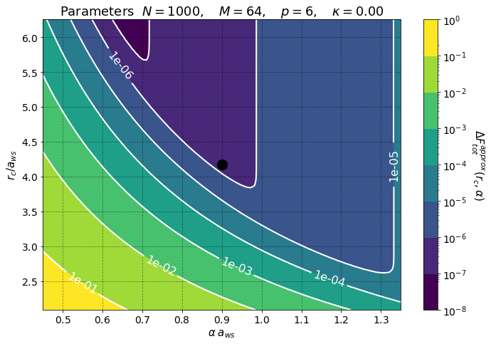
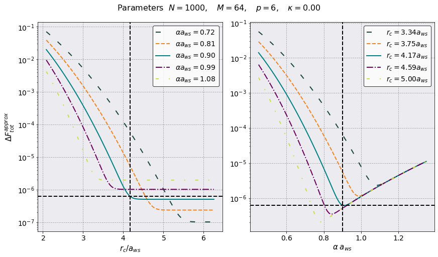
PreProcessing shows that we have chosen good parameters for the pppm algorithm. The black dot in the first plot shows our choice of parameters. This leads to a Total Force Error \(\sim 9 \times 10^8\). The horizontal and vertical lines in the above plots represent the value \(r = L/2 a_{\rm ws}\).

A common technique used in magnetized MD is to equilibrate the system in two steps. First without the presence of the magnetic field and then with the magnetic field turned on. This is because, the magnetic field can greatly delay the relaxation to equilibrium see Ott et al PRE 2017. Hence the magnetization phase before the production phase.

We confirm that our choice of parameters leads to the same physical system as the one simulated by Bernu. \(\Gamma =95\), \(\beta = 1.0\). Contrarily to Bernu we choose to run our simulation for a much longer time.

Production:
No. of production steps = 70000
Total production time = 7.7000e-13 [s] ~ 1290 w_p T_prod
snapshot interval step = 5
snapshot interval time = 5.5000e-17 [s] = 0.0922 w_p T_snap
Total number of snapshots = 14000

Bernu ran a simulation for 244 plasma periods. We decided to run for a time 5 times longer. This is because we want to show the time slicing option in the Postprocessing phase.

The estimated times, on this machine, are

----------------------- Total Estimated Times ------------------------


Equilibration Time: 0 hrs 3 min 30 sec

Magnetization Time: 0 hrs 3 min 1 sec

Production Time: 0 hrs 44 min 3 sec

Total Run Time: 0 hrs 50 min 35 sec

and the entire run requires a minimum of 132 MB of space on the hard drive.

Total minimum needed space: 2 GB 208 MB 2 KB 496 bytes

We are ready to start the simulation.

Simulation

# sim = Simulation(input_file_name)
# sim.setup(read_yaml=True)
# sim.run()

PostProcessing

postproc = PostProcess(input_file_name)
postproc.setup(read_yaml=True)

postproc.therm.setup(postproc.parameters)

postproc.therm.temp_energy_plot(postproc)
# postproc.therm.plot(scaling = 1.0e-15, y = 'Total Energy', logy = True, xlabel = r'$t$ [fs]')

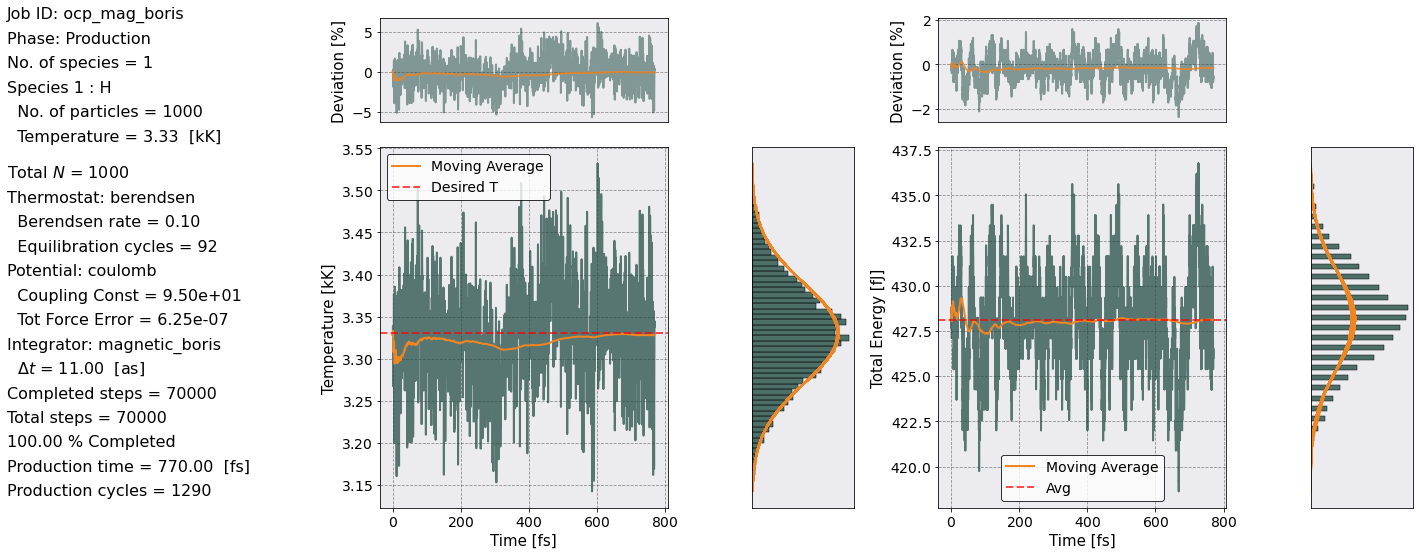
The energy remained fairly constant over the entire production phase. The Temperature similarly oscillated widly (\(\sim 5 \%\)) but its average is exactly the desired value. Both the Temperature and the Total Energy show a Gaussian distribution around their means.

We are ready to calculate the diffusion coefficient.

Transport

In the case of a magnetized plasma we have two diffusion coefficients:

\[D_{\parallel}(\tau) = \frac{k_B T}{m} \int_0^\tau dt Z_{\parallel}(t), \quad D_{\perp}(\tau) = \frac{k_B T}{m} \int_0^\tau dt Z_{\perp}(t)\]

where, for the case of a constant magnetic field in the \(z\)-direction

\[Z_{\parallel}(t) = \langle v_z(t)v_z(0) \rangle, \quad Z_{\perp}(t) = \frac{1}{2} \left [ \langle v_x(t)v_x(0) \rangle + \langle v_y(t)v_y(0) \rangle \right ],\]

are the velocity autocorrelation functions. These functions are calculated by the class VelocityAutocorrelationFunction in sarkas.tools.observables. This class calculates and saves \(Z(t)\) for each axis and the total \(Z(t) = \frac{1}{3} \left [ Z_x(t) + Z_y(t) + Z_z(t) \right ]\).

Transport coefficient are calculated using the TransportCoefficients class from the sarkas.tools.transport. This method requires the parameters of the simulation passed as postproc.parameters. The phase argument in this case is not needed since production is the default phase, and the number of slices in which to divide the simulation,no_slices. As mentioned above we decided to run our simulation 5 times longer than Bernu’s. This is because we wanted to divide our long simulation into 5 small simulations of length ~ 258 \(\omega_p T\) (Bernu’s was 244 \(\omega_p T\)), calculate the diffusion coefficients for each of them, and average them.

Sarkas was created with this workflow in mind and the option no_slices allows to do exactly this.

Once the class is imported the diffusion coefficiey calling the method diffusion. This method takes care of calnt is calculated bculating the perpendicular and parallel diffusion coefficients, and plot their averages with a shaded area.

It is important to note that the diffusion method assume a constant magnetic field in the \(z\)-direction. Arbitrary directions of the magnetic field are not supported at the moment.

from sarkas.tools.observables import VelocityAutoCorrelationFunction
from sarkas.tools.transport import TransportCoefficients

vacf = VelocityAutoCorrelationFunction()
vacf.setup(postproc.parameters, phase = 'production', no_slices = 5)
#vacf.compute()
vacf.parse()

tc = TransportCoefficients(postproc.parameters, phase = 'production', no_slices = 5)
tc.diffusion(vacf)

======================= Diffusion Coefficient ========================

Data saved in:
 Simulations/ocp_mag_boris/PostProcessing/TransportCoefficients/Production/Diffusion_ocp_mag_boris.h5
Simulations/ocp_mag_boris/PostProcessing/TransportCoefficients/Production/Diffusion_slices_ocp_mag_boris.h5

No. of slices = 5
No. dumps per slice = 560
Time interval of autocorrelation function = 1.5400e-13 [s] ~ 258 w_p T

tc.diffusion_df

	Time	H Diffusion
	NaN	Parallel		Perpendicular
	NaN	Mean	Std	Mean	Std
0	0.000000e+00	0.000000e+00	0.000000e+00	0.000000e+00	0.000000e+00
1	5.500000e-17	0.000000e+00	0.000000e+00	0.000000e+00	0.000000e+00
2	1.100000e-16	1.513632e-09	1.449843e-11	1.500904e-09	9.712383e-12
3	1.650000e-16	3.022980e-09	2.899158e-11	2.985556e-09	1.927020e-11
4	2.200000e-16	4.523784e-09	4.346764e-11	4.437928e-09	2.852923e-11
...	...	...	...	...	...
2795	1.537250e-13	1.317944e-08	2.338327e-09	9.956043e-09	1.893927e-09
2796	1.537800e-13	1.315739e-08	2.371333e-09	9.951686e-09	1.899606e-09
2797	1.538350e-13	1.313432e-08	2.404148e-09	9.946636e-09	1.905537e-09
2798	1.538900e-13	1.311026e-08	2.436658e-09	9.940771e-09	1.911840e-09
2799	1.539450e-13	1.308527e-08	2.468751e-09	9.933983e-09	1.918634e-09

2800 rows × 5 columns

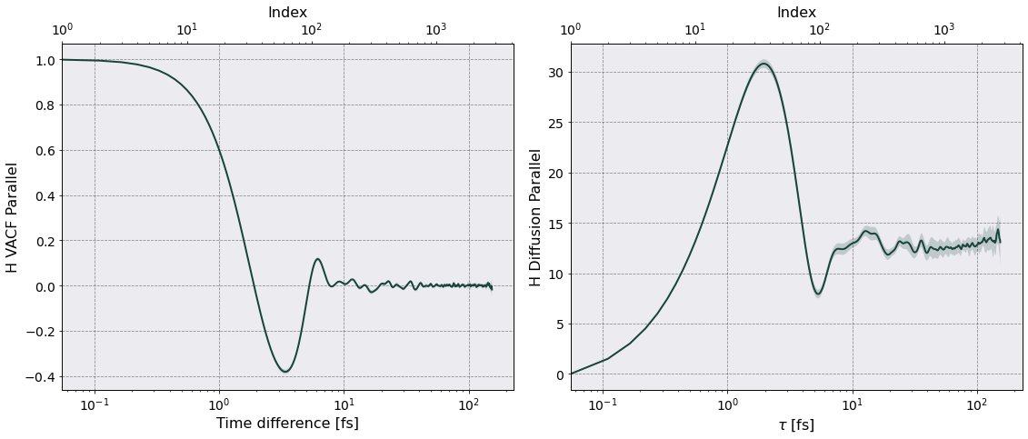
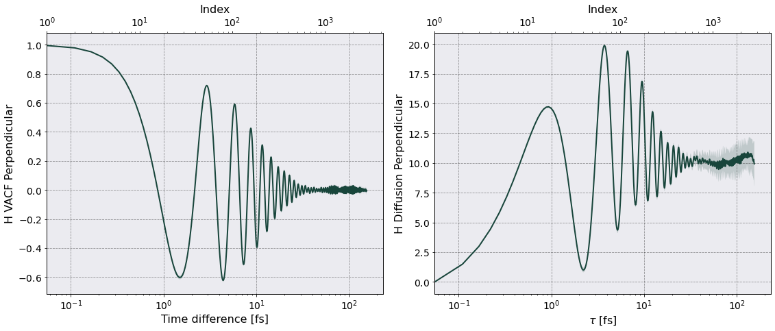
Once the calculation is complete Sarkas produces a figure for each diffusion coefficient containing two subplots: a plot of \(Z_{\parallel}(t)(Z_{\perp}(t) )\) on the left and a plot of \(D_{\parallel}(\tau)\) \((D_{\perp}(\tau))\) on the right. The above plots are in mks units, let’s rescale by \(\omega_p a_{\rm ws}^2\).

rescaling = postproc.parameters.total_plasma_frequency * postproc.parameters.a_ws**2
fig, ax = plt.subplots(1,1, figsize=(10,7))
ax2 = ax.twiny()
ax.plot(tc.diffusion_df["Time"].iloc[:,0]*1e15, tc.diffusion_df[("H Diffusion", "Parallel","Mean")]/rescaling,
       label = r'$D_{\parallel}$')
ax.fill_between(
    tc.diffusion_df["Time"].iloc[:,0]*1e15,
    tc.diffusion_df[("H Diffusion", "Parallel","Mean")]/rescaling - tc.diffusion_df[("H Diffusion", "Parallel","Std")]/rescaling,
    tc.diffusion_df[("H Diffusion", "Parallel","Mean")]/rescaling + tc.diffusion_df[("H Diffusion", "Parallel","Std")]/rescaling,
    alpha = 0.2)

# Perpendicular
ax.plot(tc.diffusion_df["Time"].iloc[:,0]*1e15, tc.diffusion_df[("H Diffusion", "Perpendicular","Mean")]/rescaling,
        label = r'$D_{\perp}$')
ax.fill_between(
    tc.diffusion_df["Time"].iloc[:,0]*1e15,
    tc.diffusion_df[("H Diffusion", "Perpendicular","Mean")]/rescaling - tc.diffusion_df[("H Diffusion", "Perpendicular","Std")]/rescaling,
    tc.diffusion_df[("H Diffusion", "Perpendicular","Mean")]/rescaling + tc.diffusion_df[("H Diffusion", "Perpendicular","Std")]/rescaling,
    alpha = 0.2)

ax.plot(tc.diffusion_df["Time"].iloc[:,0]*1e15, tc.diffusion_df[("H Diffusion", "Parallel","Mean")].expanding().mean()/rescaling,
       ls = '--', label = 'Mov Avg')

ax.plot(tc.diffusion_df["Time"].iloc[:,0]*1e15, tc.diffusion_df[("H Diffusion", "Perpendicular","Mean")].expanding().mean()/rescaling,
        ls = '--', label = r'Mov Avg')
# ax.axhline(coefficient["H Parallel Diffusion avg"].iloc[10]/rescaling)
# ax2.plot(diffusion["H Parallel Diffusion avg"].expanding().mean()/rescaling, ls = '')
# ax.grid(False)
ax.legend(ncol = 2)
ax.set_xlim(tc.diffusion_df["Time"].iloc[1,0]*1e15, 1.5*tc.diffusion_df["Time"].iloc[-1,0]*1e15)
_ = ax.set( xlabel = r'$\tau$ [fs]', ylabel =r'$D_{\parallel,\perp}$ [$\omega_p a_{ws}^2$]', xscale = 'log')

ax2.set_xlim([1,1500*1.5])
ax2.grid(alpha = 0.1)
ax2.set( xscale = 'log', xlabel = 'Index')

[None, Text(0.5, 0, 'Index')]

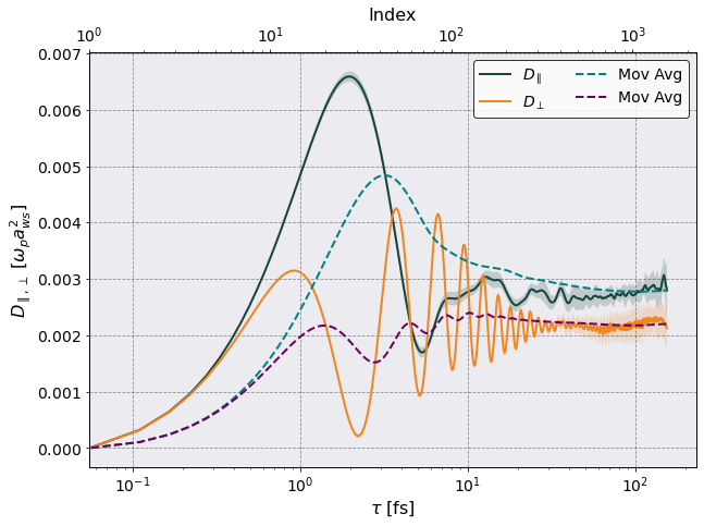
This gives a clearer picture of the diffusion coefficient. Note that the diffusion is a constant and not a function of time. This plot is meant to show how the diffusion changes as the upper limit of the time integration is varied. The final value to be published would be an average over the last ~ 800 diffusion values.

print('The perpendicular diffusion is D_x = {:.4f} w_p a_ws^2'.format(
    1/rescaling * tc.diffusion_df["H Diffusion","Perpendicular","Mean"].iloc[-800:].mean()) )
print('The parallel diffusion is D_z = {:.4f} w_p a_ws^2'.format(
    1/rescaling * tc.diffusion_df["H Diffusion","Parallel","Mean"].iloc[-800:].mean()) )

The perpendicular diffusion is D_x = 0.0023 w_p a_ws^2
The parallel diffusion is D_z = 0.0029 w_p a_ws^2