MD for Experiment Validation#

The YAML input file can be found at input_file and this notebook at notebook.

Ultracold Neutral Plasmas#

Sarkas has been developed with the experimental plasma physics community in mind. An example of strongly coupled plasmas are Ultracold Neutral Plasmas. In these systems a cloud of \(N \sim 10^6 - 10^9\) neutral atoms is trapped and cooled to ~mK temperatures. The cloud has a spherical Gaussian density distribution with peak densities in the range \(\sim 10^{15}-10^{16}\, \textrm{N/cc}\) with a standard deviation ranging from hundreds of \(\mu\)m to few mm. A portion of the atoms is then ionized by shining a laser, with the correct wavelength, onto the cloud. The energy from the laser is deposited on the electrons which now have enough energy to escape the the atoms, thus, leaving behind positively charged ions.

UNPs are an optimal experimental setup to study strongly coupled plasmas since the charge number, the number density, and the temperature of the plasma are well defined and controllable. This is in contrast to other experiments in which some parameters are not well known and require simulations and models to be extracted from experimental data.

UNPs are considered strongly coupled plasmas because of their low kinetic energy. The strong coupling parameter is defined as

\[\Gamma = \frac{(Ze)^2}{4\pi \varepsilon_0 a_{\rm ws}} \frac{1}{k_B T}\]

where \(Z\) is the charge number of the ions, \(T\) their temperature, and \(a = (3/ 4\pi n)^{1/3}\) is the Wigner-Seitz radius defined by the number density \(n\). In UNP experiments \(1 < \Gamma \sim 10\).

Disorder Induced Heating#

In the laser-cooling phase of the experiment atoms are neutral. This allows them to get very close to each other and distribute randomly in space. The potential energy in this case is very low and so is the kinetic energy. By photoionizing the atoms we are effectively turning on the Coulomb interaction. The system now has a large potential energy which pushes the ions apart, thus the potential energy is converted into kinetic energy (\(\sim k_BT\)). This process is called Disorder Induced Heating (DIH).

DIH is unavoidable and it is one of the biggest obstacles that prevents UNPs to reach \(\Gamma > 10\). This is because the initial potential energy is what determines the final temperature and the final \(\Gamma\). Large potential energies lead to large kinetic energies and low \(\Gamma\). Furthermore, in an experiment the temperature evolution of the ions in the DIH phase is used to determine/validate the number density of the initial charged cloud.

In the following example we will present a workflow to prepare and run an MD simulation and extract the DIH temperature of a UNP.

PreProcessing#

We start by importing the usual libraries and creating a path to the input file of our simulation.

[1]:

%pylab
%matplotlib inline
import os
import pandas as pd

from sarkas.processes import PreProcess, Simulation, PostProcess

plt.style.use('MSUstyle')
input_file = os.path.join('input_files', 'ucp_N10k.yaml')

Using matplotlib backend: Qt5Agg
Populating the interactive namespace from numpy and matplotlib

We then run the PreProcess.run() method to validate our simulation parameters.

[7]:

# Initialize the class
preproc = PreProcess(input_file)
# Setup Sarkas classes and initialize all the parameters
preproc.setup(read_yaml=True)
# Run 100 steps to calculate the total time of the simulation.
# Also show plots of the Force error to validate the PPPM parameters.
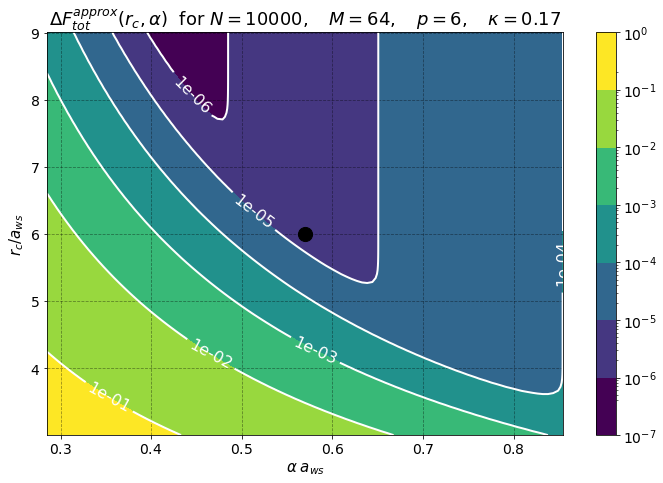
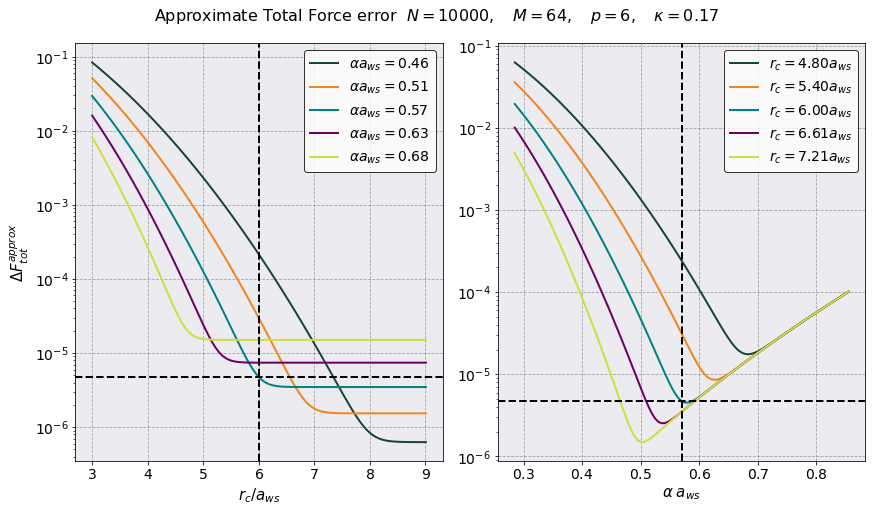
preproc.run(loops = 15, pppm_estimate = True)






 _______              __
|     __|.---.-.----.|  |--.---.-.-----.
|__     ||  _  |   _||    <|  _  |__ --|
|_______||___._|__|  |__|__|___._|_____|



An open-source pure-python molecular dynamics code for non-ideal plasmas.



* * * * * * * * * * * * * * * * * * * * * * * * * * * * * * * * * * * * * * * * * * * * * * * * * *
                                 Preprocessing
* * * * * * * * * * * * * * * * * * * * * * * * * * * * * * * * * * * * * * * * * * * * * * * * * *

Job ID:  ucp_N10k
Job directory:  UCP_DIH_N10k/ucp_N10k
Equilibration dumps directory:  UCP_DIH_N10k/ucp_N10k/PreProcessing/Equilibration/dumps
Production dumps directory:  UCP_DIH_N10k/ucp_N10k/PreProcessing/Production/dumps
Random Seed =  651951

PARTICLES:
Total No. of particles =  10000
No. of species =  1
Species ID: 0
        Name: Sr
        No. of particles = 10000
        Number density = 4.000000e+15 [N/m^3]
        Atomic weight = 88.0000 [a.u.]
        Mass = 1.471907e-25 [kg]
        Mass density = 5.887629e-10 [kg/m^3]
        Charge number/ionization degree = 1.0000
        Charge = 1.602177e-19 [C]
        Temperature = 2.000000e-03 [K] = 1.723467e-07 [eV]
        Debye Length = 4.879672e-08 [Hz]
        Plasma Frequency = 8.876174e+06 [Hz]

SIMULATION BOX:
Units:  mks
Wigner-Seitz radius = 3.907963e-06 [m]
No. of non-zero box dimensions =  3
Box side along x axis = 3.472931e+01 a_ws = 1.357209e-04 [m]
Box side along y axis = 3.472931e+01 a_ws = 1.357209e-04 [m]
Box side along z axis = 3.472931e+01 a_ws = 1.357209e-04 [m]
Box Volume = 2.500000e-12 [m^3]
Boundary conditions: periodic

ELECTRON PROPERTIES:
Number density: n_e = 4.000000e+15 [N/m^3]
Wigner-Seitz radius: a_e = 3.907963e-06 [m]
Temperature: T_e = 4.300000e+02 [K] = 3.705453e-02 [eV]
de Broglie wavelength: lambda_deB = 3.594560e-09 [m]
Thomas-Fermi length: lambda_TF = 2.262611e-05 [m]
Fermi wave number: k_F = 4.910891e+05 [1/m]
Fermi Energy: E_F = 9.188478e-09 [eV]
Relativistic parameter: x_F = 0.000000 --> E_F = 9.190629e-09 [eV]
Degeneracy parameter: Theta = 4032717.0039
Coupling: r_s = 73849.801701,  Gamma_e = 0.009944
Warm Dense Matter Parameter: W = 0.0000
Chemical potential: mu = -23.099609 k_B T_e = -93154186.8939 E_F

THERMOSTAT:
Type: Berendsen
First thermostating timestep, i.e. relaxation_timestep = 0
Berendsen parameter tau: 5.000 [s]
Berendsen relaxation rate: 0.200 [Hz]

!!!!!!!!!!!!!!!!!!!!!!!!!!!!!!!!!! WARNING !!!!!!!!!!!!!!!!!!!!!!!!!!!!!!!!!!
Equilibration temperatures not defined. I will use the species's temperatures.
!!!!!!!!!!!!!!!!!!!!!!!!!!!!!!!!!!!!!!!!!!!!!!!!!!!!!!!!!!!!!!!!!!!!!!!!!!!!!!

Thermostating temperatures:
Species ID 0: T_eq = 2.000000e-03 [K] = 1.723467e-07 [eV]

POTENTIAL:  Yukawa
electron temperature = 4.3000e+02 [K] = 3.7055e-02 [eV]
kappa = 0.1727
Gamma_eff = 2137.95

ALGORITHM:  P3M
Mesh = 64 x 64 x 64
Ewald parameter alpha = 0.5700 / a_ws = 1.458560e+05 [1/m]
Mesh width = 0.5426, 0.5426, 0.5426 a_ws
           = 2.1206e-06, 2.1206e-06, 2.1206e-06 [m]
Mesh size * Ewald_parameter (h * alpha) = 0.3093, 0.3093, 0.3093
                                        ~ 1/3, 1/3, 1/3
rcut = 6.0050 a_ws = 2.346716e-05 [m]
No. of PP cells per dimension =  5,  5,  5
No. of particles in PP loop =   1395
No. of PP neighbors per particle =    216
PM Force Error = 3.482296e-06
PP Force Error = 3.181860e-06
Tot Force Error = 4.717056e-06

INTEGRATOR:
Type: Verlet
Time step = 3.019042e-10 [s]
Total plasma frequency = 8.876174e+06 [Hz]
w_p dt = 0.0027

Equilibration:
No. of equilibration steps = 0
Total equilibration time = 0.0000e+00 [s] ~ 0 w_p T_eq
snapshot interval step = 5
snapshot interval time = 1.5095e-09 [s] = 0.0134 w_p T_snap
Total number of snapshots = 0

Production:
No. of production steps = 10000
Total production time = 3.0190e-06 [s] ~ 26 w_p T_prod
snapshot interval step = 5
snapshot interval time = 1.5095e-09 [s] = 0.0134 w_p T_snap
Total number of snapshots = 2000


------------------------ Initialization Times ------------------------


Potential Initialization Time: 0 hrs 0 min 3 sec

Particles Initialization Time: 0 sec 1 msec 821 usec 58 nsec

Total Simulation Initialization Time: 0 hrs 0 min 3 sec


========================== Times Estimates ===========================

Optimal Green's Function Time:
0 min 3 sec 713 msec 803 usec 454 nsec

Time of PP acceleration calculation averaged over 15 steps:
0 min 0 sec 252 msec 560 usec 197 nsec

Time of PM acceleration calculation averaged over 15 steps:
0 min 0 sec 6 msec 4 usec 525 nsec


Running 15 equilibration and production steps to estimate simulation times


Time of a single equilibration step averaged over 15 steps:
0 min 0 sec 310 msec 992 usec 655 nsec


Time of a single production step averaged over 15 steps:
0 min 0 sec 313 msec 249 usec 470 nsec



----------------------- Total Estimated Times ------------------------


Equilibration Time: 0 sec 0 msec 0 usec 0 nsec

Production Time: 0 hrs 52 min 12 sec

Total Run Time: 0 hrs 52 min 12 sec


========================= Filesize Estimates =========================


Equilibration:

Checkpoint filesize: 0 GB 0 MB 860 KB 822 bytes
Checkpoint folder size: 0 GB 0 MB 0 KB 0 bytes

Production:

Checkpoint filesize: 0 GB 0 MB 860 KB 822 bytes
Checkpoint folder size: 1 GB 657 MB 261 KB 480 bytes

Total minimum needed space: 1 GB 657 MB 261 KB 480 bytes

../../_images/examples_UNP_UCP_Experiment_Validation_4_5.png

../../_images/examples_UNP_UCP_Experiment_Validation_4_6.png

Simulation#

Once the simulation parameters have been decided we can start running our simulation. Since we are dealing with a non-equilibrium simulation, in order to get some statistics we need to run multiple simulations with different initial conditions. This can be done by changing the random number seed.

Below we show a sample code that executes three (3) MD simulation by changing only the rand_seed parameter and the storing directory.

[9]:

# Define a random number generator
rg = np.random.Generator( np.random.PCG64(154245) )

# Loop over the number of independent MD runs to perform
for i in range(5):
    # Get a new seed
    seed = rg.integers(0, 15198)

    args = {
        "Parameters": {"rand_seed": seed}, # define a new rand_seed for each simulation

        "IO":   # Store all simulations' data in simulations_dir,
                # but save the dumps in different subfolders (job_dir)
            {
                "simulations_dir": 'UCP_DIH_N10k',
                "job_dir": "run{}".format(i),
                "verbose": False # This is so not to print to screen for every run
            },
    }
    # Run the simulation.
    sim = Simulation(input_file)
    sim.setup(read_yaml=True, other_inputs=args)
    sim.run()
    print('Run {} completed'.format(i) )

Run 0 completed
Run 1 completed
Run 2 completed
Run 3 completed
Run 4 completed

The above code will take a long time, because we need to wait for the previous simulation to finish before starting a new one. Notice that we define the rand_seed parameter in each loop. This is because even though we are in the same Python process Sarkas has a default rand_seed. Thus, if we don’t pass it we will end up with three identical simulations.

If we can afford to occupy few processors on our computer we can save time by running each simulation in a different JupyterNotebook or by running three Python scripts at the same time.

PostProcessing#

Once the simulations are done, we can start our Post Processing. In the following we will calculate the average temperature and RMS speed of each species in the mixture. Save them into a pandas.DataFrame and plot them.

[2]:

# Initialize the storing df
Temp_vel_data = pd.DataFrame()

# No. of independent runs
runs = 5

# Loop over the runs and initialize the PostProcess
for i in range(runs):
    # This is a copy-n-paste from the code snippet above. We only change sim with postproc
    # Some lines are commented out because they are not needed.

    # Get a new seed
    #seed = rg.integers(0, 1598765198)

    args = {
        # "Parameters": {"rand_seed": seed}, # define a new rand_seed for each simulation

        "IO":   # Store all simulations' data in simulations_dir,
                # but save the dumps in different subfolders (job_dir)
            {
                "simulations_dir": 'UCP_DIH_N10k',
                "job_dir": "run{}".format(i),
                "verbose": False  # This is so not to print to screen for every run
            },
    }

    postproc = PostProcess(input_file)
    postproc.setup(read_yaml = True, other_inputs=args)

    # Rename the Thermodynamics class for convenience
    E = postproc.therm
    # Setup its attributes
    E.setup(postproc.parameters)
    # Grab the data
    E.parse()

    # Save the time array once. Obviously this has to be the same for each run.
    if i == 0:
        Temp_vel_data['Time'] = E.dataframe["Time"] * 1e6 # scale by microsec

    # Grab the total temperature. This is the only line needed in the case of a One-Component plasma
    Temp_vel_data['Temperature run {}'.format(i)] = E.dataframe["Temperature"]
    Temp_vel_data['Gamma run {}'.format(i)] = E.qe**2/ (E.fourpie0 * E.kB * E.a_ws * E.dataframe['Temperature'])
    Temp_vel_data['RMS Speed run {}'.format(i)] = np.sqrt(E.kB * E.dataframe['Temperature'] / postproc.species[0].mass)

[3]:

# Let's look at the data
Temp_vel_data.head(10)

[3]:

	Time	Temperature run 0	Gamma run 0	RMS Speed run 0	Temperature run 1	Gamma run 1	RMS Speed run 1	Temperature run 2	Gamma run 2	RMS Speed run 2	Temperature run 3	Gamma run 3	RMS Speed run 3	Temperature run 4	Gamma run 4	RMS Speed run 4
0	0.000000	0.002012	2125.666966	0.434378	0.001992	2147.003605	0.432214	0.001993	2145.592909	0.432356	0.002012	2125.365953	0.434409	0.002005	2132.681082	0.433663
1	0.001510	0.009476	451.222732	0.942801	0.006148	695.477531	0.759406	0.009681	441.675962	0.952936	0.012002	356.270734	1.061025	0.003814	1121.000474	0.598154
2	0.003019	0.023311	183.432031	1.478693	0.016799	254.530966	1.255294	0.022098	193.493293	1.439735	0.021207	201.626702	1.410398	0.009698	440.910836	0.953763
3	0.004529	0.038579	110.834706	1.902294	0.029746	143.745577	1.670392	0.035179	121.547016	1.816534	0.031782	134.538921	1.726600	0.018777	227.720617	1.327133
4	0.006038	0.054996	77.749003	2.271267	0.043874	97.458663	2.028642	0.049228	86.859581	2.148853	0.043945	97.301324	2.030282	0.030239	141.405760	1.684155
5	0.007548	0.072377	59.078500	2.605559	0.058923	72.567377	2.350958	0.064311	66.487554	2.456097	0.057549	74.299751	2.323389	0.043533	98.223216	2.020731
6	0.009057	0.090588	47.201953	2.914980	0.074789	57.172839	2.648627	0.080374	53.200328	2.745734	0.072451	59.017560	2.606904	0.058304	73.337758	2.338578
7	0.010567	0.109529	39.039205	3.205274	0.091403	46.780602	2.928079	0.097322	43.935660	3.021392	0.088517	48.306028	2.881476	0.074312	57.539937	2.640164
8	0.012076	0.129121	33.115612	3.480160	0.108710	39.333349	3.193267	0.115059	37.162774	3.285198	0.105623	40.482759	3.147608	0.091377	46.793979	2.927660
9	0.013586	0.149300	28.639787	3.742232	0.126656	33.760134	3.446780	0.133493	32.030846	3.538600	0.123657	34.578691	3.405739	0.109361	39.099164	3.202815

[4]:

# Calculate mean and std using a loop

tags = ["Temperature", "Gamma", "RMS Speed"]

for lbl in tags:

    # Average Temperature
    mean_tot = Temp_vel_data[ ["{} run {}".format(lbl, i) for i in range(runs) ]].mean( axis = 1)
    std_tot = Temp_vel_data[ ["{} run {}".format(lbl, i) for i in range(runs) ]].std( axis = 1)

    # Average and Standard Deviation of Total Temperature
    Temp_vel_data['Mean {}'.format(lbl)] = mean_tot
    Temp_vel_data['Std {}'.format(lbl)] = std_tot

# Save the data
file_path = os.path.join(postproc.io.simulations_dir,'Temp_vel_data.csv')
Temp_vel_data.to_csv(file_path, index=False, encoding='utf-8')

# Let's look at the data again but only at the last additions
Temp_vel_data.iloc[:10, 16:]

[4]:

	Mean Temperature	Std Temperature	Mean Gamma	Std Gamma	Mean RMS Speed	Std RMS Speed
0	0.002003	0.000010	2135.262103	10.502982	0.433404	0.001065
1	0.008224	0.003229	613.129486	310.765453	0.862864	0.183402
2	0.018623	0.005561	254.798766	107.606476	1.307576	0.215196
3	0.030813	0.007522	147.677368	46.462825	1.688591	0.220492
4	0.044456	0.009173	100.154866	24.473638	2.032640	0.219039
5	0.059339	0.010582	74.131280	14.730142	2.351347	0.215456
6	0.075301	0.011797	57.986087	9.703094	2.650965	0.211079
7	0.092217	0.012852	47.120286	6.810584	2.935277	0.206369
8	0.109978	0.013773	39.377695	5.008591	3.206779	0.201543
9	0.128493	0.014584	33.621724	3.817325	3.467233	0.196745

It is now time to plot and compare with experiment. For this tutorial we grabbed experimental data from Fig.~(2) of this paper. This data was obtained using WebPlotDigitizer and saved into the file paper_data.csv.

We will plot both the temperature and the RMS speed side by side and compare with the experimental data.

[12]:

# Grab data from Killian
paper_data = np.loadtxt('paper_data.csv', delimiter=',')

# Plot Temperature and thermal speed
fig, (ax_temp, ax_rms) = plt.subplots(1,2, figsize=(16, 7))

# Plot Temperature
Temp_vel_data.plot(x = 'Time', y = 'Mean Temperature', ax = ax_temp)
# Plot std error as shaded area
ax_temp.fill_between(
    Temp_vel_data['Time'],
    Temp_vel_data["Mean Temperature"] - Temp_vel_data["Std Temperature"],
    Temp_vel_data["Mean Temperature"] + Temp_vel_data["Std Temperature"],
    alpha = 0.2)
# Plot paper data
ax_temp.scatter(paper_data[:,0], paper_data[:,1], s=100, label = 'Paper Data')
# embellish
ax_temp.grid(alpha = 0.3)
ax_temp.legend()
ax_temp.set(ylabel = r'$T$ [K]', xlabel =r'Time [$\mu$s]')

# Plot Gamma
# Temp_vel_data.plot(x = 'Time', y = 'Mean Gamma', ax = ax_gamma)
# ax_gamma.fill_between(
#     Temp_vel_data['Time'],
#     Temp_vel_data["Mean Gamma"] - Temp_vel_data["Std Gamma"],
#     Temp_vel_data["Mean Gamma"] + Temp_vel_data["Std Gamma"], alpha = 0.2)

# ax_gamma.grid(alpha = 0.3)
# ax_gamma.set(ylabel = r'$\Gamma$', xlabel =r'Time [$\mu$s]', ylim = (0, 5))

# Plot RMS Speed
Temp_vel_data.plot(x = 'Time', y = 'Mean RMS Speed', ax = ax_rms)
# Plot std error as shaded area
ax_rms.fill_between(
    Temp_vel_data['Time'],
    Temp_vel_data["Mean RMS Speed"] - Temp_vel_data["Std RMS Speed"],
    Temp_vel_data["Mean RMS Speed"] + Temp_vel_data["Std RMS Speed"], alpha = 0.2)

# embellish
ax_rms.grid(alpha = 0.3)
ax_rms.set( ylabel = r'$v$ [m/s]', xlabel= r'Time [$\mu$s]')

# Finishing
fig.tight_layout()
figname = os.path.join(postproc.io.simulations_dir,'Temperature_n_RMS_Plot.png')
fig.savefig(figname)

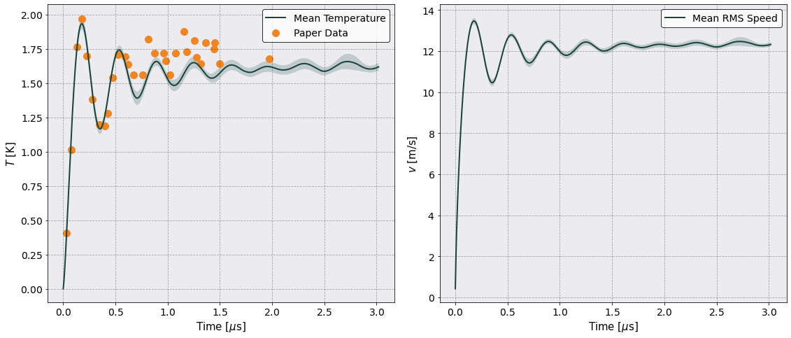
../../_images/examples_UNP_UCP_Experiment_Validation_13_0.png

Noice! There is good agreement for the first microsecond.

Distributions for Thermalization analysis#

The next important quantity that we need are velocity distributions. Sarkas allows you to calculate these easily and automatically average of the multiple runs and over the three cartesian dimensions. The last two are flags that can be passed when calculating.

First we print the parameters of the velocity distributions

[15]:

from sarkas.tools.observables import VelocityDistribution

vd = VelocityDistribution()
vd.setup(
    postproc.parameters, # We need to pass simulations parameters always
    max_no_moment=10, # This is the maximum number of distribution moments to calculate
    multi_run_average=True, # Do we want to average over multiple runs ?
    runs = 5, # Tell me the number of runs.
    dimensional_average=True, # Do we want to average over the three directions?
    max_hermite_order = 5
)

# Let's print out some info
vd.pretty_print()



======================= Velocity Distribution ========================

CSV dataframe saved in:
          UCP_DIH_N10k/PostProcessing/Production/VelocityDistribution/VelocityDistribution.csv
HDF5 dataframe saved in:
          UCP_DIH_N10k/PostProcessing/Production/VelocityDistribution/VelocityDistribution.h5
Data accessible at: self.dataframe, self.hierarchical_dataframe, self.species_bin_edges

Multi run average:  True
No. of runs:  5
Size of the parsed velocity array: 2001 x 1 x 150000

Histograms Information:
Species: Sr
No. of samples = 150000
Thermal speed: v_th = 1.207819e+01 [m/s]
density: True
bins: 200
range : ( -5.00, 5.00 ) v_th,
        ( -6.0391e+01, 6.0391e+01 ) [m/s]
Bin Width = 0.0500

Moments Information:
CSV dataframe saved in:
          UCP_DIH_N10k/PostProcessing/Production/VelocityDistribution/Moments_run4.csv
Data accessible at: self.moments_dataframe, self.moments_hdf_dataframe
Highest moment to calculate: 10

Grad Expansion Information:
CSV dataframe saved in:
          UCP_DIH_N10k/PostProcessing/Production/VelocityDistribution/HermiteCoefficients_run4.csv
Data accessible at: self.hermite_dataframe, self.hermite_hdf_dataframe
Highest order to calculate: 5
RMS Tolerance: 0.050

[16]:

# Let's get the thermal speed of each species
vd.vth

# Create a dictionary with the input arguments accepted by np.histogram
hist_kwargs = {
    'range': [ # In a multispecies case you need to pass a list
        (-13*vd.vth[0],13*vd.vth[0]),
    ],
    'bins': [
        520,
    ]
}

# Reassign the attributes with the new dictionary
vd.setup(
    postproc.parameters, # We need to pass simulations parameters always
    max_no_moment=10, # This is the maximum number of distribution moments to calculate
    multi_run_average=True, # Do we want to average over multiple runs ?
    runs = 5, # Tell me the number of runs.
    dimensional_average=True, # Do we want to average over the three directions?
    max_hermite_order = 5,
    hist_kwargs= hist_kwargs, # < === Here is the new dictionary
)

# Let's print it again
vd.pretty_print()



======================= Velocity Distribution ========================

CSV dataframe saved in:
          UCP_DIH_N10k/PostProcessing/Production/VelocityDistribution/VelocityDistribution.csv
HDF5 dataframe saved in:
          UCP_DIH_N10k/PostProcessing/Production/VelocityDistribution/VelocityDistribution.h5
Data accessible at: self.dataframe, self.hierarchical_dataframe, self.species_bin_edges

Multi run average:  True
No. of runs:  5
Size of the parsed velocity array: 2001 x 1 x 150000

Histograms Information:
Species: Sr
No. of samples = 150000
Thermal speed: v_th = 1.207819e+01 [m/s]
range : ( -13.00, 13.00 ) v_th,
        ( -1.5702e+02, 1.5702e+02 ) [m/s]
bins: 520
density: True
Bin Width = 0.0500

Moments Information:
CSV dataframe saved in:
          UCP_DIH_N10k/PostProcessing/Production/VelocityDistribution/Moments_run4.csv
Data accessible at: self.moments_dataframe, self.moments_hdf_dataframe
Highest moment to calculate: 10

Grad Expansion Information:
CSV dataframe saved in:
          UCP_DIH_N10k/PostProcessing/Production/VelocityDistribution/HermiteCoefficients_run4.csv
Data accessible at: self.hermite_dataframe, self.hermite_hdf_dataframe
Highest order to calculate: 5
RMS Tolerance: 0.050

[17]:

# Let's finally calculate the distributions
vd.compute()



======================= Velocity Distribution ========================

CSV dataframe saved in:
          UCP_DIH_N10k/PostProcessing/Production/VelocityDistribution/VelocityDistribution.csv
HDF5 dataframe saved in:
          UCP_DIH_N10k/PostProcessing/Production/VelocityDistribution/VelocityDistribution.h5
Data accessible at: self.dataframe, self.hierarchical_dataframe, self.species_bin_edges

Multi run average:  True
No. of runs:  5
Size of the parsed velocity array: 2001 x 1 x 150000

Histograms Information:
Species: Sr
No. of samples = 150000
Thermal speed: v_th = 1.207819e+01 [m/s]
range : ( -13.00, 13.00 ) v_th,
        ( -1.5702e+02, 1.5702e+02 ) [m/s]
bins: 520
density: True
Bin Width = 0.0500

Moments Information:
CSV dataframe saved in:
          UCP_DIH_N10k/PostProcessing/Production/VelocityDistribution/Moments_run4.csv
Data accessible at: self.moments_dataframe, self.moments_hdf_dataframe
Highest moment to calculate: 10

Grad Expansion Information:
CSV dataframe saved in:
          UCP_DIH_N10k/PostProcessing/Production/VelocityDistribution/HermiteCoefficients_run4.csv
Data accessible at: self.hermite_dataframe, self.hermite_hdf_dataframe
Highest order to calculate: 5
RMS Tolerance: 0.050

Collecting data from snapshots ...

Creating velocity distributions ...

Velocity distribution calculation Time: 0 hrs 0 min 3 sec

Calculating velocity moments ...

Velocity moments calculation Time: 0 hrs 0 min 16 sec

Calculating Hermite coefficients ...

/home/luciano/Documents/Programming/sarkas/sarkas/tools/observables.py:3292: RuntimeWarning: invalid value encountered in true_divide
  ratios[:, :, :, mom] = moments[:, :, :, mom] / (const * moments[:, :, :, 1] ** (pwr / 2.))

/home/luciano/anaconda3/envs/sarkas/lib/python3.7/site-packages/scipy/optimize/minpack.py:829: OptimizeWarning: Covariance of the parameters could not be estimated
  category=OptimizeWarning)




Hermite expansion calculation Time: 0 hrs 0 min 22 sec

MD for Experiment Validation

Content