
Data Analysis
Content
Data Analysis#
Once the simulation is complete we enter the Post Processing stage where we measure physical quantities and calculate transport coefficients.
Sarkas was developed to make this process as simple and straightforward as possible.
The YAML input file can be found at input_file and this notebook at notebook
Let’s import the needed packages.
[1]:
# Import the usual libraries
%pylab
%matplotlib inline
import os

plt.style.use('MSUstyle')

# Import sarkas
from sarkas.processes import PostProcess

# Create the file path to the YAML input file
input_file_name = os.path.join('input_files', 'yukawa_mks_p3m.yaml')
Using matplotlib backend: Qt5Agg
Populating the interactive namespace from numpy and matplotlib
Similar to the Pre Processing and Simulation stages three lines are enough. The run method will calculate everything that was included in the input YAML file. This was shown in the Quickstart notebook where we calculated the Radial Distribution Function. In this notebook we want to calculate the Radial Distribution Function and the Static Structure Function.
Each observable is an object and it is stored as an attribute of the PostProcess. The class names are
therm = Thermodynamics
rdf = Radial Distribution Function
ssf = Static Structure Factor
Other class names that we are not calculating here are:
dsf = Dynamic Structure Function
ccf = Current Correlation Function
ec = Electric Current
vacf = Velocity AutoCorrelation Function
diff_flux = Flux AutoCorrelation Function ( mixtures only)
p_tensor = Pressure Tensor
You can find more information for each observable on the Observable page and our Examples page for more info on how to use them.
Let’s run the postprocessing
[2]:
# Let's initialize the class
postproc = PostProcess(input_file_name)
postproc.setup(read_yaml=True)
postproc.run()
==================== Radial Distribution Function ====================

Data saved in:
 Simulations/yocp_pppm/PostProcessing/RadialDistributionFunction/Production/RadialDistributionFunction_yocp.h5
Data accessible at: self.ra_values, self.dataframe

No. bins = 500
dr = 0.0110 a_ws = 1.2540e-13 [m]
Maximum Distance (i.e. potential.rc)= 5.5100 a_ws = 6.2702e-11 [m]
Radial Distribution Function Calculation Time: 0 sec 57 msec 85 usec 789 nsec


===================== Static Structure Function ======================

k wavevector information saved in:
 Simulations/yocp_pppm/PostProcessing/k_space_data/k_arrays.npz
n(k,t) Data saved in:
 Simulations/yocp_pppm/PostProcessing/k_space_data/nkt.h5
Data saved in:
 Simulations/yocp_pppm/PostProcessing/StaticStructureFunction/Production/StaticStructureFunction_yocp.h5
Data accessible at: self.k_list, self.k_counts, self.ka_values, self.dataframe

Smallest wavevector k_min = 2 pi / L = 3.9 / N^(1/3)
k_min = 0.1809 / a_ws = 1.5898e+10 [1/m]

Angle averaging choice: custom
        Maximum angle averaged k harmonics = n_x, n_y, n_z = 13, 13, 13
        Largest angle averaged k_max = k_min * sqrt( n_x^2 + n_y^2 + n_z^2)
        AA k_max = 4.0737 / a_ws = 3.5798e+11 [1/m]
        Maximum k harmonics = n_x, n_y, n_z = 66, 66, 66
        Largest wavector k_max = k_min * n_x
        k_max = 11.9406 / a_ws = 1.0493e+12 [1/m]

Total number of k values to calculate = 2902
No. of unique ka values to calculate = 427

Calculating n(k,t) for slice 1/2.
Calculating n(k,t) for slice 2/2.
n(k,t) Calculation Time: 0 hrs 29 min 10 sec

Calculating S(k) ...
Static Structure Function Calculation Time: 0 sec 346 msec 697 usec 472 nsec
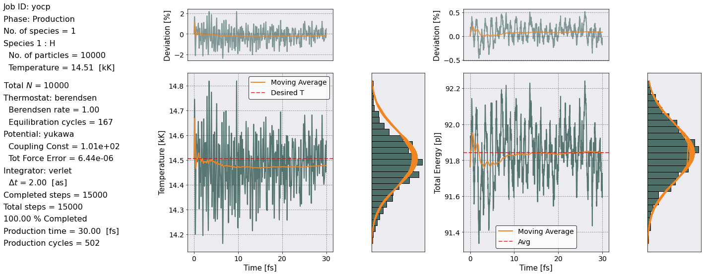
As you can see Sarkas calculated the Radial distribution function, the Static structure function, and produced a plot of the temperature and energy of the production phase.
On the left most part of the figure above we reproduce some useful info. The main plots show the Temperature (left) and Total Energy (right) as a function of time. The temperature plot shows the thermostating temperature as a red dashed line. In the energy plot, instead, the red dashed line represents the average value. The yellow-orange line shows the moving average.
The plots above the main plots indicate the percentage deviation from the desired temperature (left) and the percentage deviation of the total energy from its initial value. Also in these plots, the yellow-orange line shows the moving average of the percentage deviation.
The bar plots to the right of the main plots instead are histograms of the Temperature and Total Energy, respectively.
Note that the Temperature oscillates around its desired value and has only \(\sim \pm 2\)% deviation from it. Similarly the Total Energy oscillates around its average value and stays within a \(\sim -0.5\) % deviation.
The bar plots are the next most important thing to notice. We want these to look like Maxwellian distributions. The orange line in the Temperature bar plot is a Maxwellian distribution with a centered at the desired Temperature (dashed red line) with a standard deviation obtained from the actual data. The orange line in the Energy bar plot is again a Maxwellian distribution centered at the dashed red line with a std equal to \(k_BT\).
Thermodynamics#
We can create a similar plot for the equilibration phase by calling the method temp_energy_plot
[3]:
postproc.therm.temp_energy_plot(
    postproc, # Pass the Process class with simulation info
    phase = 'equilibration' # Choose the simulation phase
)
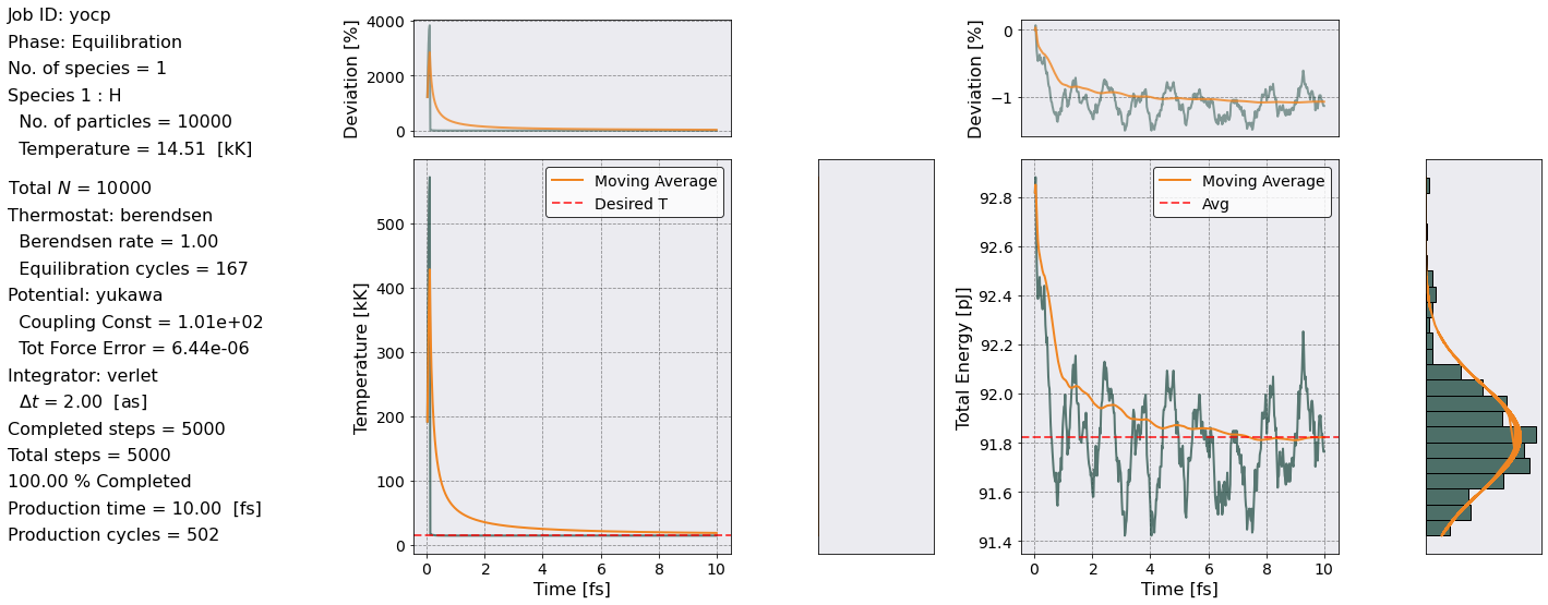
We find a figure similar as before. In this case, the most important thing to pay attention to is the temperature plot. We want to see that the Moving Average has approached the desired temperature.
Radial Distribution Function#
The RDF has been already calculated and the data saved on disk in the directory displayed above.
As mentioned in the output the data is stored in a pandas.DataFrame(). Let’s take a look
[4]:
postproc.rdf.dataframe
[4]:
| Distance | H-H RDF | ||
|---|---|---|---|
| NaN | Mean | Std | |
| 0 | 0.000000e+00 | 0.000000 | NaN |
| 1 | 1.881060e-13 | 0.000000 | NaN |
| 2 | 3.135100e-13 | 0.000000 | NaN |
| 3 | 4.389140e-13 | 0.000000 | NaN |
| 4 | 5.643180e-13 | 0.000000 | NaN |
| ... | ... | ... | ... |
| 495 | 6.213768e-11 | 0.962613 | NaN |
| 496 | 6.226309e-11 | 0.962260 | NaN |
| 497 | 6.238849e-11 | 0.962209 | NaN |
| 498 | 6.251389e-11 | 0.962449 | NaN |
| 499 | 6.263930e-11 | 0.962889 | NaN |
500 rows × 3 columns
This is a pandas.DataFrame with MultiIndex. There are two rows of columns this means that columns of data are called via tuples, e.g. postproc.rdf.dataframe[("H-H RDF", "Mean")]
As you can see there are three columns. The first is the distance between two particles and it is given in the same units as provided in the YAML. The next two columns are the Mean and Std of the RDF calculated for each slice. The Std column is full of NaN because we only had one slice as such no std.
Let’s plot it!. This can be done by calling the plot() method of the Observable class. We reproduce here the docs for convenience
def plot(self, scaling=None, acf=False, longitudinal=True, figname=None, show=False, **kwargs):
    """
    Plot the observable by calling the pandas.DataFrame.plot() function and save the figure.

    Parameters
    ----------
    scaling : float, tuple
        Factor by which to rescale the x and y axis.

    acf : bool
        Flag for renormalizing the autocorrelation functions. Default= False

    longitudinal : bool
        Flag for longitudinal plot in case of CurrenCurrelationFunction. Default = True

    figname : str
        Name with which to save the file. It automatically saves it in the correct directory.

    show : bool
        Flag for prompting the plot to screen. Default=False

    **kwargs :
        Options to pass to matplotlib plotting method.

    Returns
    -------
    axes_handle : matplotlib.axes.Axes
        Axes. See `pandas` documentation for more info

    """
This method takes the first column of the dataframe as the \(x\) axis and all the other columns as \(y\) axis. As you can see this method is a wrapper for the pandas.DataFrame.plot() method, as such you can pass the same parameters. We have added other parameters specific for our plots. In particular the parameter scaling is used for rescaling the \(x\) and \(y\) axis.
In the following we want to plot the RDF as a function of \(r/a_{ws}\) and relabel the x-axis.
[5]:
# Plot
postproc.rdf.plot(
    scaling=postproc.rdf.a_ws,
    xlabel = r'$r/a_{ws}$')
[5]:
<AxesSubplot:xlabel='$r/a_{ws}$'>
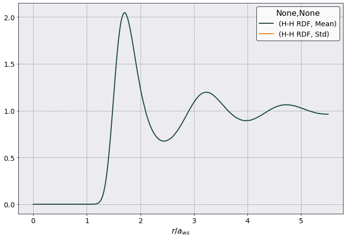
Nice!
Static Structure Factor#
The next observable we want to measure is the Static Structure Factor. Here you can find a long Wikipedia article about it. In short it is the correlation function of the density fluctuations and Sarkas calculates it by
For each timestep Sarkas calculates
then takes the product \(n(-\mathbf k,t) n(\mathbf k,t)\) and averages over the time length of each slice
where \(M\) is the total number of saved (slice) timesteps and \(\Delta t\) is our snapshot timestep.
Notice that \(\mathbf k\) is a vector, as such there are multiple directions we need to consider. The first important thing to understand is that even though we are using periodic boundary conditions to simulate an infinite system, the number of wavelengths that can fit into the simulation box are finite and given by
where \(n_{x,y,z}\) can take only integer values. This means that the minimum value is
with $ L = L_x = L_y = L_z$. The calculation of \(S(\mathbf k)\) for every combination of the triplet \(n_x, n_y, n_z\) can be very slow. Therefore, it is often the case that researchers calculate only multiple integers of \(k_{\rm min}\) along the three principal axis, that is
This is the default way in Sarkas and it corresponds to the choice angle_averaging = 'principal_axis'. If we wanted to calculate every possible combination of the triplet then we would choose angle_averaging = 'full'.
In the YAML file we passed the value angle_averaging = 'custom', in order to show this feature. Sarkas calculated \(S(\mathbf k)\) up to \(ka = 12\), where \(a = a_{\rm ws}\) for brevity. It calculated every possible combination of the triplet up to max_aa_ka_value = 4.1 and then used multiples of the principal axis for the rest.
Same as before let’s take a look at the data
[6]:
postproc.ssf.dataframe
[6]:
| Inverse Wavelength | H-H SSF | ||
|---|---|---|---|
| NaN | Mean | Std | |
| 0 | 1.589833e+10 | 0.020323 | 0.010770 |
| 1 | 2.248364e+10 | 0.009977 | 0.005976 |
| 2 | 2.753672e+10 | 0.011418 | 0.003642 |
| 3 | 3.179666e+10 | 0.001656 | 0.001383 |
| 4 | 3.554975e+10 | 0.003375 | 0.001673 |
| ... | ... | ... | ... |
| 422 | 9.856965e+11 | 0.999040 | 0.002366 |
| 423 | 1.001595e+12 | 1.095194 | 0.015077 |
| 424 | 1.017493e+12 | 0.960260 | 0.018005 |
| 425 | 1.033392e+12 | 0.966948 | 0.064647 |
| 426 | 1.049290e+12 | 1.004454 | 0.052012 |
427 rows × 3 columns
Note that in this case the Std column is not NaN, because we have chosen to divide the simulation into two slices.
As you can see Sarkas will calculate 2902 different combinations which correspond to 427 unique values of \(ka\). This means that our \(S(k)\) will be an array with 427 elements.
Let’s compute it! Again a progress bar will show up in your notebook, but does not display on the webpage.
[7]:
postproc.ssf.parse()
As you can see Sarkas calculates \(n(\mathbf k, t)\) first for each slice, only one in this case. This is the slow part of the calculation. Then computes \(S(k)\) by averaging over all the configurations.
Let’s take a look at the dataframe
[8]:
postproc.ssf.dataframe
[8]:
| Inverse Wavelength | H-H SSF | ||
|---|---|---|---|
| NaN | Mean | Std | |
| 0 | 1.589833e+10 | 0.020323 | 0.010770 |
| 1 | 2.248364e+10 | 0.009977 | 0.005976 |
| 2 | 2.753672e+10 | 0.011418 | 0.003642 |
| 3 | 3.179666e+10 | 0.001656 | 0.001383 |
| 4 | 3.554975e+10 | 0.003375 | 0.001673 |
| ... | ... | ... | ... |
| 422 | 9.856965e+11 | 0.999040 | 0.002366 |
| 423 | 1.001595e+12 | 1.095194 | 0.015077 |
| 424 | 1.017493e+12 | 0.960260 | 0.018005 |
| 425 | 1.033392e+12 | 0.966948 | 0.064647 |
| 426 | 1.049290e+12 | 1.004454 | 0.052012 |
427 rows × 3 columns
Let’s plot it! This time, though, let’s plot also the std as a shaded area around the mean.
[9]:
# Get the axes handle for the errorbar plot
ax = postproc.ssf.plot(
    scaling = 1./postproc.ssf.a_ws, # Need to divide because a_ws multiplies k
    y = ('H-H SSF', "Mean"), # I want only the second column. Otherwise it will plot all the columns
    xlabel = r'$ka$'
)
# Errorbar plot
ax.fill_between(
    postproc.ssf.dataframe[('Inverse Wavelength')].iloc[:,0] * postproc.ssf.a_ws,
    postproc.ssf.dataframe[("H-H SSF", "Mean")] + postproc.ssf.dataframe[("H-H SSF", "Std")],
    postproc.ssf.dataframe[("H-H SSF", "Mean")] - postproc.ssf.dataframe[("H-H SSF", "Std")],
    alpha = 0.2
)
ax.set(ylim = (0, 3))
[9]:
[(0.0, 3.0)]
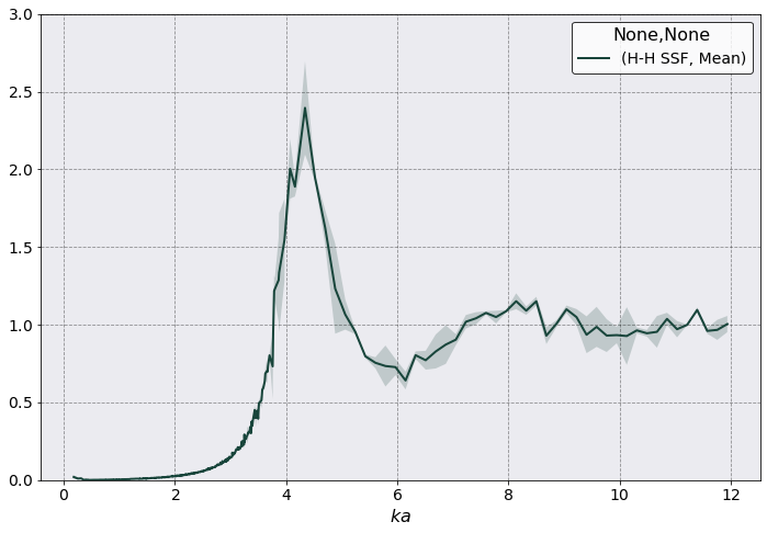
As you can see \(S(\mathbf k)\) is quite noisy for \(ka > 4.0\). There are two reasons for this.
Slice averaging
Angle averaging
Slice averaging it actually not that significant here and it contributes only to the shaded areas. As a matter of fact notice how smooth is the plot for \(ka < 4.0\).
Principal axis averaging is the culprit here. For each \(k\) value there are only \(3 \times 1500\) configuration on which to average, where \(1500\) is the number of snapshots and \(3\) comes from the three principal directions of \(k\). For example \(ka = 6.15\) corresponds to the three directions
To reduce the noise we could choose among: increasing the number of snapshots, use the angle_averaging = 'full', or increasing the number of particles. All these options are rather slow. More importantly we don’t know which is the most effective.
Probably, angle_averaging = 'full' will be more effective for the large \(ka\) value, but it definitely won’t reduce any noise at low \(ka\) values. However, assuming we don’t want to restart the simulation (i.e. increase the number of particles) let’s take a look at what it would take to do the full angle averaging.
The following code computes
[10]:
postproc.ssf.angle_averaging = 'full'
# Re-Initialize the class with the new parameters.
postproc.ssf.setup(postproc.parameters)
# Check
postproc.ssf.pretty_print()
===================== Static Structure Function ======================

k wavevector information saved in:
 Simulations/yocp_pppm/PostProcessing/k_space_data/k_arrays.npz
n(k,t) Data saved in:
 Simulations/yocp_pppm/PostProcessing/k_space_data/nkt.h5
Data saved in:
 Simulations/yocp_pppm/PostProcessing/StaticStructureFunction/Production/StaticStructureFunction_yocp.h5
Data accessible at: self.k_list, self.k_counts, self.ka_values, self.dataframe

Smallest wavevector k_min = 2 pi / L = 3.9 / N^(1/3)
k_min = 0.1809 / a_ws = 1.5898e+10 [1/m]

Angle averaging choice: full
        Maximum angle averaged k harmonics = n_x, n_y, n_z = 66, 66, 66
        Largest angle averaged k_max = k_min * sqrt( n_x^2 + n_y^2 + n_z^2)
        k_max = 20.6818 / a_ws = 1.8174e+12 [1/m]

Total number of k values to calculate = 300762
No. of unique ka values to calculate = 14344
Notice that we now have 300 762 combinations of \((n_x, n_y, n_z)\) to calculate. This will be rather slow.
[ ]: