Quantum Statistical Potential Simulation#

The YAML input file can be found at input_file and this notebook at notebook.

[1]:

# Import the usual libraries
%pylab
%matplotlib inline
import os

plt.style.use('MSUstyle')
# Import sarkas
from sarkas.processes import Simulation, PostProcess, PreProcess

# Create the file path to the YAML input file
input_file_name = os.path.join('input_files',  'QSP_cgs.yaml')

Using matplotlib backend: Qt5Agg
Populating the interactive namespace from numpy and matplotlib

[2]:

# sim = PreProcess(input_file_name)
# sim.setup(read_yaml=True)
# sim.run(loops = 20,
#     pppm_estimate=True)

[3]:

# sim = Simulation(input_file_name)
# sim.setup(read_yaml=True)
# sim.run()

[4]:

postproc = PostProcess(input_file_name)
postproc.setup(read_yaml=True)

[5]:

# Equilibration check
postproc.therm.setup(postproc.parameters)
# postproc.therm.temp_energy_plot(postproc, phase='equilibration')

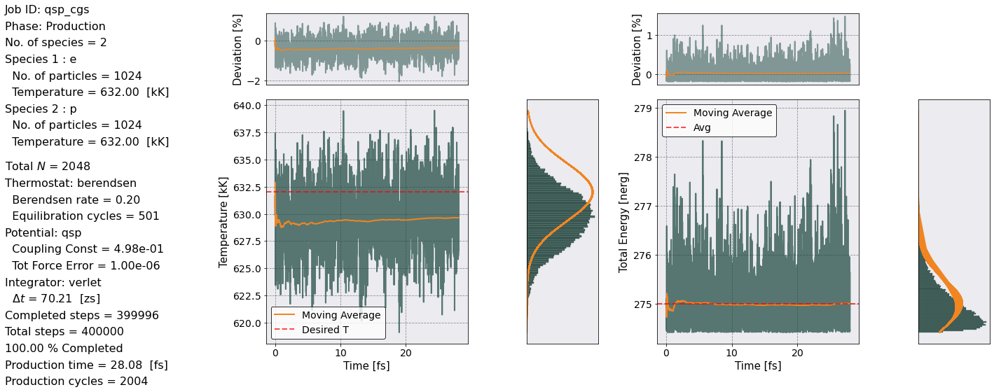
[6]:

# Production check
postproc.therm.temp_energy_plot(postproc, phase='production')

../../_images/examples_QSP_QSP_Tutorial_6_0.png

[7]:

# Radial Distribution Function
postproc.rdf.setup(postproc.parameters)
postproc.rdf.compute()
# Grab HNC data for comparison
hnc_r, hnc_gee, hnc_gei, hnc_gii = np.loadtxt('hnc_gall.out', unpack=True)


Radial Distribution Function Calculation Time: 0 sec 62 msec 25 usec 174 nsec

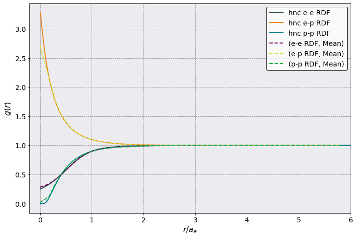
[8]:

fig, ax = plt.subplots(1,1, figsize=(10,7))
ax.plot(hnc_r , hnc_gee, label = 'hnc e-e RDF')
ax.plot(hnc_r , hnc_gei, label = 'hnc e-p RDF')
ax.plot(hnc_r , hnc_gii, label = 'hnc p-p RDF')
postproc.rdf.plot(scaling = postproc.parameters.electron_WS_radius,
                  y = [('e-e RDF', "Mean"),
                       ('e-p RDF', "Mean"),
                       ('p-p RDF', "Mean")
                      ],
                  ax = ax,
                  ls = '--')
ax.legend()
ax.set(xlim = (-0.2, 6), xlabel = r'$r/a_e$', ylabel = r"$g(r)$")

[8]:

[(-0.2, 6.0),
 Text(0.5, 135.8333333333334, '$r/a_e$'),
 Text(61.22856648763023, 0.5, '$g(r)$')]

../../_images/examples_QSP_QSP_Tutorial_8_1.png

[9]:

from sarkas.tools.observables import ElectricCurrent
from sarkas.tools.transport import TransportCoefficients

[10]:

ec = ElectricCurrent()
ec.setup(postproc.parameters, no_slices = 4)
#ec.compute()
ec.parse()

[11]:

ec.dataframe

[11]:

	Time	e Electric Current						p Electric Current						Electric Current
	NaN	X		Y		Z		X		Y		Z		X		Y		Z
	NaN	Mean	Std	Mean	Std	Mean	Std	Mean	Std	Mean	Std	Mean	Std	Mean	Std	Mean	Std	Mean	Std
0	0.000000e+00	-1.592979	4.266312	0.313781	4.696336	2.091885	4.912189	-0.000868	0.002324	0.000171	0.002558	0.001139	0.002675	-1.593846	4.268636	0.313952	4.698894	2.093025	4.914864
1	4.212480e-19	-1.556820	4.255951	0.261228	4.727619	2.129823	4.919757	-0.000848	0.002318	0.000142	0.002575	0.001160	0.002679	-1.557668	4.258269	0.261370	4.730193	2.130983	4.922436
2	8.424960e-19	-1.514293	4.250659	0.212417	4.757823	2.165856	4.927102	-0.000825	0.002315	0.000116	0.002591	0.001180	0.002683	-1.515118	4.252974	0.212533	4.760414	2.167036	4.929785
3	1.263744e-18	-1.470321	4.251131	0.169078	4.780538	2.200074	4.932380	-0.000801	0.002315	0.000092	0.002604	0.001198	0.002686	-1.471122	4.253446	0.169170	4.783142	2.201272	4.935066
4	1.684992e-18	-1.428866	4.254351	0.127651	4.795915	2.235364	4.932165	-0.000778	0.002317	0.000070	0.002612	0.001217	0.002686	-1.429644	4.256668	0.127721	4.798526	2.236581	4.934851
...	...	...	...	...	...	...	...	...	...	...	...	...	...	...	...	...	...	...	...
16661	7.018413e-15	-5.074025	6.949550	1.247491	4.710895	2.787523	4.774233	-0.002763	0.003785	0.000679	0.002566	0.001518	0.002600	-5.076789	6.953335	1.248170	4.713460	2.789041	4.776834
16662	7.018834e-15	-5.047354	6.958353	1.189807	4.720378	2.837681	4.749905	-0.002749	0.003790	0.000648	0.002571	0.001545	0.002587	-5.050103	6.962143	1.190455	4.722948	2.839226	4.752492
16663	7.019255e-15	-5.019247	6.964106	1.131542	4.733726	2.891892	4.732832	-0.002734	0.003793	0.000616	0.002578	0.001575	0.002578	-5.021981	6.967898	1.132158	4.736304	2.893467	4.735410
16664	7.019677e-15	-4.991651	6.969232	1.069791	4.753368	2.948593	4.725178	-0.002719	0.003796	0.000583	0.002589	0.001606	0.002573	-4.994370	6.973027	1.070374	4.755957	2.950199	4.727751
16665	7.020098e-15	-4.965582	6.977188	1.003926	4.777691	3.006825	4.728724	-0.002704	0.003800	0.000547	0.002602	0.001638	0.002575	-4.968286	6.980988	1.004473	4.780293	3.008462	4.731299

16666 rows × 19 columns

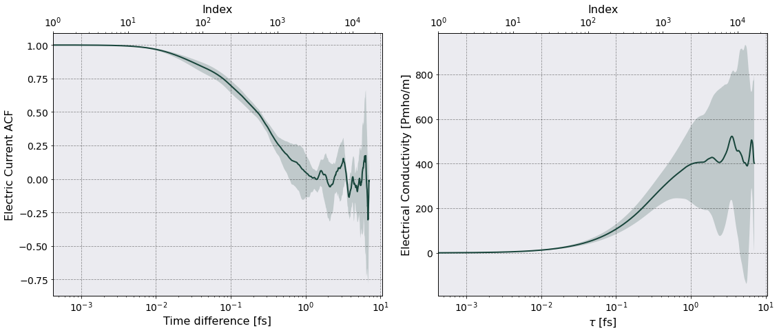
[12]:

tc = TransportCoefficients(postproc.parameters)
tc.electrical_conductivity(ec, "ElectricalConductivity")



====================== Electrical Conductivity =======================

Data saved in:
 Simulations/qsp_cgs/PostProcessing/TransportCoefficients/Production/ElectricalConductivity_qsp_cgs.h5
Simulations/qsp_cgs/PostProcessing/TransportCoefficients/Production/ElectricalConductivity_slices_qsp_cgs.h5

No. of slices = 4
No. dumps per slice = 2777
Time interval of autocorrelation function = 7.0205e-15 [s] ~ 501 w_p T

../../_images/examples_QSP_QSP_Tutorial_12_2.png

[13]:

tc.conductivity_df

[13]:

	Time	Electrical Conductivity
	NaN	Mean	Std
0	0.000000e+00	0.000000e+00	0.000000e+00
1	4.212480e-19	0.000000e+00	0.000000e+00
2	8.424960e-19	5.412416e+14	9.348701e+13
3	1.263744e-18	1.082391e+15	1.869658e+14
4	1.684992e-18	1.623361e+15	2.804388e+14
...	...	...	...
16661	7.018413e-15	4.022931e+17	3.956391e+17
16662	7.018834e-15	4.022840e+17	3.957253e+17
16663	7.019255e-15	4.022752e+17	3.958105e+17
16664	7.019677e-15	4.022667e+17	3.958949e+17
16665	7.020098e-15	4.022586e+17	3.959783e+17

16666 rows × 3 columns

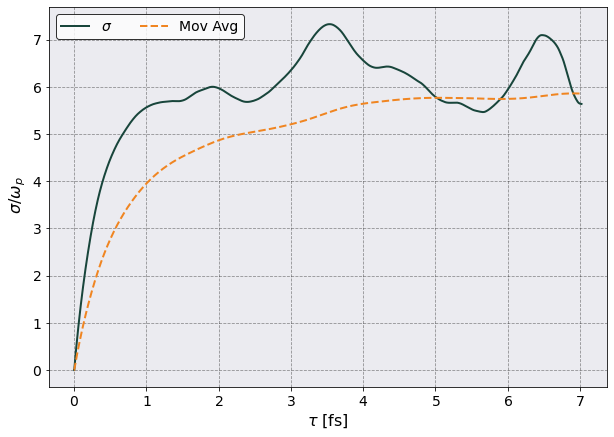
[14]:

rescaling = 1.0/ec.total_plasma_frequency
fig, ax = plt.subplots(1,1, figsize=(10,7))
ax.plot(tc.conductivity_df["Time"].iloc[:,0]*1e15,
        tc.conductivity_df[("Electrical Conductivity", "Mean")] * rescaling,
       label = r'$\sigma$')

ax.plot(tc.conductivity_df["Time"].iloc[:,0]*1e15, tc.conductivity_df[("Electrical Conductivity", "Mean")].expanding().mean() * rescaling,
        ls = '--', label = r'Mov Avg')

ax.legend(ncol = 2)
ax.set(xlabel = r"$\tau$ [fs]",ylabel = r" $\sigma/\omega_p$")

[14]:

[Text(0.5, 0, '$\\tau$ [fs]'), Text(0, 0.5, ' $\\sigma/\\omega_p$')]

../../_images/examples_QSP_QSP_Tutorial_14_1.png