
Ultrafast electron cooling in an expanding ultracold plasma
Content
Ultrafast electron cooling in an expanding ultracold plasma#
The YAML input file can be found at input_file and this notebook at notebook.
Ultracold Microplasma#
Let us observe the Ultrafast electron cooling in an expanding ultracold plasma. Here, a cloud of neutral atoms is trapped and cooled to quantum degeneracy at ~nK temperatures. The Bose-Einstein condensate (BEC) with a peak number density of \(n \sim 2 \times 10^{20}\, \textrm{m}^{-3}\) is then rapidly ionized by a femtosecond laser pulse of \(511\, \textrm{nm}\) wavelength and \(215\, \textrm{fs}\) duration so that \(N \sim 4000\) ions and electrons immediately emerge after two-photon ionization. The excess energy of \(0.68\, \textrm{eV}\) is distributed between ions and electrons leading to an initial ion temperature of \(T_{\rm i} \sim 33\, \textrm{mK}\) and fast escaping electrons of \(T_e \sim 5250\, \textrm{K}\).
The ions are initially strongly coupled as the temperture is very small compared to the Coulomb energy of the dense, ionized BEC:
where \(T_{\rm i}\) is the ion temperature, and \(a_{\rm ws} = [3 / (4\pi n)]^{1/3}\) is the Wigner-Seitz radius defined by the number density \(n\).
The high density also leads to ultrafast dynamics as the inverse electron plasma frequency is given by:
Initialization#
We start by importing the usual libraries and creating a path to the input file of our simulation.
[1]:
%pylab
%matplotlib inline
import os
import pandas as pd

from sarkas.processes import PreProcess, Simulation, PostProcess

plt.style.use('MSUstyle')
input_file = os.path.join('input_files', 'uec.yaml')
Using matplotlib backend: <object object at 0x7f8c38283720>
Populating the interactive namespace from numpy and matplotlib
Simulation#
Let us start the simulation.
[2]:
# Initialize the Simulation class
sim = Simulation(input_file)
# Setup the simulation's parameters
sim.setup(read_yaml=True)
# Run the simulation
sim.run()
__ _
/ _\ __ _ _ __| | ____ _ ___
\ \ / _` | '__| |/ / _` / __|
_\ \ (_| | | | < (_| \__ \
\__/\__,_|_| |_|\_\__,_|___/
An open-source pure-python molecular dynamics suite for non-ideal plasmas.
* * * * * * * * * * * * * * * * * * * * * * * * * * * * * * * * * * * * * * * * * * * * * * * * * *
Simulation
* * * * * * * * * * * * * * * * * * * * * * * * * * * * * * * * * * * * * * * * * * * * * * * * * *
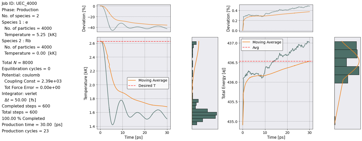
Job ID: UEC_4000
Job directory: Simulations/UEC_4000
Equilibration dumps directory:
{'Simulations/UEC_4000/Simulation/Equilibration/dumps'}
Production dumps directory:
{'Simulations/UEC_4000/Simulation/Production/dumps'}
Equilibration Thermodynamics file:
Simulations/UEC_4000/Simulation/Equilibration/EquilibrationEnergy_UEC_4000.csv
Production Thermodynamics file:
Simulations/UEC_4000/Simulation/Production/ProductionEnergy_UEC_4000.csv
PARTICLES:
Total No. of particles = 8000
No. of species = 2
Species ID: 0
Name: e
No. of particles = 4000
Number density = 2.000000e+20 [N/m^3]
Atomic weight = 5.446170e-04 [a.u.]
Mass = 9.109384e-31 [kg]
Mass density = 1.821877e-10 [kg/m^3]
Charge number/ionization degree = -1.0000
Charge = -1.602177e-19 [C]
Temperature = 5.250000e+03 [K] = 4.524100e-01 [eV]
Debye Length = 3.535658e-07 [m]
Plasma Frequency = 7.978230e+11 [rad/s]
Species ID: 1
Name: Rb
No. of particles = 4000
Number density = 2.000000e+20 [N/m^3]
Atomic weight = 8.700000e+01 [a.u.]
Mass = 1.455181e-25 [kg]
Mass density = 2.910362e-05 [kg/m^3]
Charge number/ionization degree = 1.0000
Charge = 1.602177e-19 [C]
Temperature = 3.300000e-02 [K] = 2.843720e-06 [eV]
Debye Length = 8.864364e-10 [m]
Plasma Frequency = 1.996147e+09 [rad/s]
SIMULATION AND INITIAL PARTICLE BOX:
Units: mks
No. of non-zero box dimensions = 3
Wigner-Seitz radius = 8.419452e-08 [m]
Box side along x axis = 2.375452e+03 a_ws = 2.000000e-04 [m]
Box side along y axis = 2.375452e+03 a_ws = 2.000000e-04 [m]
Box side along z axis = 2.375452e+03 a_ws = 2.000000e-04 [m]
Box Volume = 8.000000e-12 [m^3]
Initial particle box side along x axis = 2.579187e+01 a_ws = 2.171534e-06 [m]
Initial particle box side along y axis = 2.579187e+01 a_ws = 2.171534e-06 [m]
Initial particle box side along z axis = 5.037475e+01 a_ws = 4.241278e-06 [m]
Initial particle box Volume = 2.000000e-17 [m^3]
Boundary conditions: absorbing
Equilibration:
No. of equilibration steps = 0
Total equilibration time = 0.0000e+00 [s] ~ 0 w_p T_eq
snapshot interval step = 10
snapshot interval time = 5.0000e-13 [s] = 0.3989 w_p T_snap
Total number of snapshots = 0
Production:
No. of production steps = 600
Total production time = 3.0000e-11 [s] ~ 23 w_p T_eq
snapshot interval step = 4
snapshot interval time = 2.0000e-13 [s] = 0.1596 w_p T_snap
Total number of snapshots = 150
POTENTIAL: coulomb
Short-range Cutoff radius: a_rs = 2.000000e-08 [m]
Effective coupling constant: Gamma_eff = 2386.77
ALGORITHM: pp
rcut = 1187.7258 a_ws = 1.000000e-04 [m]
No. of PP cells per dimension = [2 2 2]
No. of particles in PP loop = 10800000000
No. of PP neighbors per particle = 1675516081
Tot Force Error = 0.000000e+00
INTEGRATOR:
Equilibration Integrator Type: verlet
Production Integrator Type: verlet
Time step = 5.000000e-14 [s]
Total plasma frequency = 7.978255e+11 [rad/s]
w_p dt = 0.0399 ~ 1/25
-------------------------Initialization Times-------------------------
Potential Initialization Time: 0 sec 14 msec 697 usec 371 nsec
Particles Initialization Time: 0 sec 1 msec 747 usec 688 nsec
Total Simulation Initialization Time: 0 sec 14 msec 697 usec 371 nsec
------------------------------Production------------------------------
/home/luciano/Documents/Programming/sarkas/sarkas/sarkas/potentials/core.py:523: AlgorithmWarning: Use the PP method with care for pure Coulomb interactions.
  warn("Use the PP method with care for pure Coulomb interactions.", category=AlgorithmWarning)
/home/luciano/Documents/Programming/sarkas/sarkas/sarkas/potentials/core.py:416: AlgorithmWarning:
Short-range cut-off enabled. Use this feature with care!
  warn("\nShort-range cut-off enabled. Use this feature with care!", category=AlgorithmWarning)
Production Time: 0 hrs 15 min 51 sec

Total Time: 0 hrs 15 min 51 sec
Notice that we are getting a Warning. This is because we are using the linked cell list (LCL) algorithm for a bare Coulomb potential. The linked cell list algorithm calculates the forces between pair of particles that are within a sphere of radius \(r_c\), i.e. the cutoff radius shown above. The Coulomb potential is a long range interaction therefore by using the LCL algorithm we are neglecting the long range portion of the force. For the purpose of this simulation we can neglect the long range part.
PostProcessing#
Now let’s have a look at the results and run the PostProcessing
[3]:
# Initialize the Postprocessing class
postproc = PostProcess(input_file)
# Read the simulation's parameters and assign attributes
postproc.setup(read_yaml=True)
# Calculate observables
postproc.run()
* * * * * * * * * * * * * * * * * * * * * * * * * * * * * * * * * * * * * * * * * * * * * * * * * *
                                 Postprocessing
* * * * * * * * * * * * * * * * * * * * * * * * * * * * * * * * * * * * * * * * * * * * * * * * * *

Job ID: UEC_4000
Job directory: Simulations/UEC_4000
PostProcessing directory:
Simulations/UEC_4000/PostProcessing

Equilibration dumps directory: Simulations/UEC_4000/Simulation/Equilibration/dumps
Production dumps directory:
Simulations/UEC_4000/Simulation/Production/dumps

Equilibration Thermodynamics file:
Simulations/UEC_4000/Simulation/Equilibration/EquilibrationEnergy_UEC_4000.csv
Production Thermodynamics file:
Simulations/UEC_4000/Simulation/Production/ProductionEnergy_UEC_4000.csv
Let us have a closer look at the energy evolution over time which we can extract from our Sarkas simulation into a pandas.DataFrame.
[4]:
# Rename the Thermodynamics class for convenience
E = postproc.therm
# Setup its attributes
E.setup(postproc.parameters)
# Grab the data
E.parse()

# Results dataframe
Temp_vel_data = pd.DataFrame()
# Time
Temp_vel_data['Time'] = E.dataframe["Time"] * 1e12 # scale by picosec
# Total energies
eVpp = 1 / (np.abs(E.qe) * postproc.species[0].num) # scale by eV per particle
Temp_vel_data['Total Energy'] = E.dataframe["Total Energy"] * eVpp
Temp_vel_data['Total Kinetic Energy'] = E.dataframe["Total Kinetic Energy"] * eVpp
Temp_vel_data['Potential Energy'] = E.dataframe["Potential Energy"] * eVpp
# Kinetic energies
Temp_vel_data['e Kinetic Energy'] = E.dataframe[' '.join([postproc.species[0].name, 'Kinetic Energy'])] * eVpp
Temp_vel_data['Ion Kinetic Energy'] = E.dataframe[' '.join([postproc.species[1].name, 'Kinetic Energy'])] * eVpp
# Potential energies
Temp_vel_data['ee Potential Energy'] = E.dataframe[' '.join([postproc.species[0].name, 'Potential Energy'])] * eVpp
Temp_vel_data['IonIon Potential Energy'] = E.dataframe[' '.join([postproc.species[1].name, 'Potential Energy'])] * eVpp
Temp_vel_data['eIon Potential Energy'] = Temp_vel_data['Potential Energy'] \
    - Temp_vel_data['ee Potential Energy'] - Temp_vel_data['IonIon Potential Energy']
It is now time to plot and compare. For this tutorial we grabbed data from Fig. 4f of this paper. The data was obtained using WebPlotDigitizer and saved into the files Ee.csv, Ei.csv and Ekinp.csv in the folder uec_data, reflecting the ultrafast energy evolution for the electrons, ions and plasma electrons, respectively.
We will compare the results with our simulation. The ion energy \(E_{\rm i}\) is composed of \(E_{\rm i} = E^{\rm kin}_{\rm i} + E^{\rm pot}_{\rm ii} + 0.5 E^{\rm pot}_{\rm ei}\) while the electron energy \(E_{\rm e}\) is composed of \(E_{\rm e} = E^{\rm kin}_{\rm e} + E^{\rm pot}_{\rm ee} + 0.5 E^{\rm pot}_{\rm ei}\) so that the inter-species potential energy \(E^{\rm pot}_{\rm ei}\) is equally shared by the electrons and ions.
[5]:
# Read paper data
Ee = pd.read_csv(os.path.join('uec_data/', 'Ee.csv'), names=['Time', 'Energy'])
Ei = pd.read_csv(os.path.join('uec_data/', 'Ei.csv'), names=['Time', 'Energy'])
Ekinp = pd.read_csv(os.path.join('uec_data/', 'Ekinp.csv'), names=['Time', 'Energy'])

# Plot
fig_energy, (ax_etot) = plt.subplots(1, 1, figsize=(10, 7))

# Simulation data
plt.plot(Temp_vel_data['Time'], Temp_vel_data['Total Energy'], linestyle='--', color='black', label='Total Energy')
ion_energy = Temp_vel_data['Ion Kinetic Energy'] + Temp_vel_data['IonIon Potential Energy'] \
             + 0.5*Temp_vel_data['eIon Potential Energy']
electron_energy = Temp_vel_data['e Kinetic Energy'] + Temp_vel_data['ee Potential Energy'] \
             + 0.5*Temp_vel_data['eIon Potential Energy']
plt.plot(Temp_vel_data['Time'], electron_energy, linestyle='-', color='skyblue', label='Electron Energy')
plt.plot(Temp_vel_data['Time'], ion_energy, linestyle='-', color='firebrick', label='Ion Energy')

# Paper data
plt.scatter(Ekinp['Time'], Ekinp['Energy'], marker='x', color='cadetblue', alpha=0.5, label=r'$E_{\rm kin,plasma}$')
plt.scatter(Ee['Time'], Ee['Energy'], marker='.', color='skyblue', alpha=0.5, label=r'$E_{\rm e}$')
plt.scatter(Ei['Time'], Ei['Energy'], marker='o', color='firebrick', alpha=0.5, label=r'$E_{\rm i}$')

plt.xlim((0, 30))
plt.ylim((0, 0.8))
ax_etot.legend()
ax_etot.set(xlabel =r'Time (ps)', ylabel = 'Energy (eV)')
fig_energy.tight_layout()
fig_energy.savefig(os.path.join(postproc.io.postprocessing_dir,'Energy_Plot.png'))
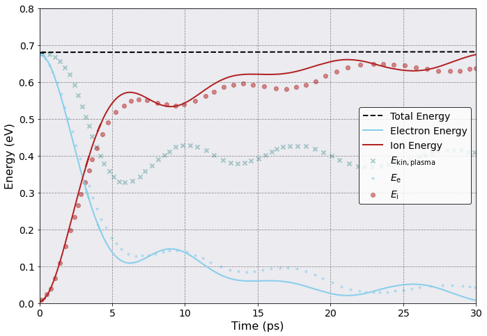
Nice! Sarkas accurately reproduces the ultrafast electron cooling. Minor descrepancies in the amplitude and electron plasma frequency are attributed to the initial particle distribution which is an elongated box in sarkas and a cylinder in the original publication.
MD Movie#
Let’s make a movie of our simulation. Running the following cell allows you to create XYZ files that can be read by Ovito to make nice MD movies.
[6]:
sim.io.dump_xyz()
We have uploaded the video on the Sarkas channel on YouTube. You can watch it by running the following cell or by copying the video id.
[7]:
from IPython.display import YouTubeVideo
YouTubeVideo("AxP1R5WQOCk",width=800,height=450)
[7]: