Yukawa vs Egs potential

In this notebook I will show a tutorial on how to run Sarkas to compare EGS and Yukawa potential. I will run one simulation per potential choice and compute the radial distribution function \(g(r)\) and the static structure factor \(S(k)\).

The good thing about Sarkas is that I can put all of this into literally few lines.

The YAML input file can be found at input_file and this notebook at notebook.

# Import the usual packages.
%pylab
%matplotlib inline
import os
import pandas as pd

from sarkas.processes import PreProcess, Simulation, PostProcess

# Set the plotting style
plt.style.use('MSUstyle')

# Link to the input file.
input_file = os.path.join('input_files', 'yukawa_egs_cgs.yaml')

Using matplotlib backend: Qt5Agg
Populating the interactive namespace from numpy and matplotlib

PreProcessing

The first thing to do is to check our simulation parameters. I use this preprocessing mainly to check if my force error is too large. Other would like to check other parameters, e.g. kappa.

# Run the simulation.
args = {
    "Potential": {"type": 'egs'},
    "IO":   # Store all simulations' data in simulations_dir,
            # but save the dumps in different subfolders (job_dir)
        {
            "simulations_dir": 'SMT',
            "job_dir": "{}_pot".format("egs")
#                 "verbose": False # This is so not to print to screen for every run
        },
}

pre = PreProcess(input_file)
pre.setup(read_yaml=True, other_inputs=args)
pre.run(loops=50, postprocessing=True)

     _______.     ___      .______       __  ___      ___           _______.
    /       |    /   \     |   _  \     |  |/  /     /   \         /       |
   |   (----`   /  ^  \    |  |_)  |    |  '  /     /  ^  \       |   (----`
    \   \      /  /_\  \   |      /     |    <     /  /_\  \       \   \
.----)   |    /  _____  \  |  |\  \----.|  .  \   /  _____  \  .----)   |
|_______/    /__/     \__\ | _| `._____||__|\__\ /__/     \__\ |_______/



An open-source pure-python molecular dynamics code for non-ideal plasmas.



* * * * * * * * * * * * * * * * * * * * * * * * * * * * * * * * * * * * * * * * * * * * * * * * * *
                                      Preprocessing
* * * * * * * * * * * * * * * * * * * * * * * * * * * * * * * * * * * * * * * * * * * * * * * * * *

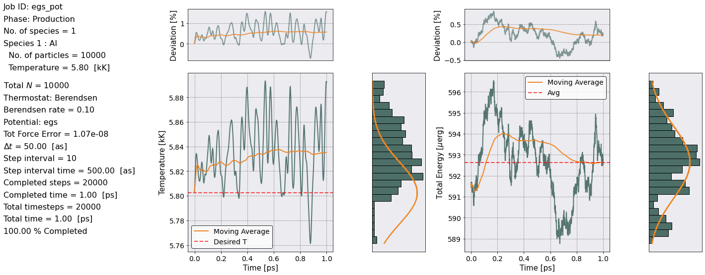
Job ID:  egs_pot
Job directory:  SMT/egs_pot
Equilibration dumps directory:  SMT/egs_pot/PreProcessing/Equilibration/dumps
Production dumps directory:  SMT/egs_pot/PreProcessing/Production/dumps
Random Seed =  13546565

PARTICLES:
Total No. of particles =  10000
No. of species =  1
Species ID: 0
        Name: Al
        No. of particles = 10000
        Number density = 6.000000e+22 [N/cc]
        Atomic weight = 26.9815 [a.u.]
        Mass = 4.512991e-23 [g]
        Mass density = 2.707795e+00 [g/cc]
        Charge number/ionization degree = 3.0000
        Charge = 1.440961e-09 [esu]
        Temperature = 5.802259e+03 [K] = 5.000000e-01 [eV]
        Debye Length = 7.153314e-10 [Hz]
        Plasma Frequency = 1.862519e+14 [Hz]

SIMULATION BOX:
Units:  cgs
Wigner-Seitz radius = 1.584601e-08 [cm]
No. of non-zero box dimensions =  3
Box side along x axis = 3.472931e+01 a_ws = 5.503212e-07 [cm]
Box side along y axis = 3.472931e+01 a_ws = 5.503212e-07 [cm]
Box side along z axis = 3.472931e+01 a_ws = 5.503212e-07 [cm]
Box Volume = 1.666667e-19 [cm^3]
Boundary conditions: periodic

ELECTRON PROPERTIES:
Number density: n_e = 1.800000e+23 [N/cc]
Wigner-Seitz radius: a_e = 1.098701e-08 [cm]
Temperature: T_e = 5.802259e+03 [K] = 5.000000e-01 [eV]
de Broglie wavelength: lambda_deB = 9.785463e-08 [cm]
Thomas-Fermi length: lambda_TF = 4.881607e-09 [cm]
Fermi wave number: k_F = 1.746752e+08 [1/cm]
Fermi Energy: E_F = 1.162479e+01 [eV]
Relativistic parameter: x_F = 0.006745 --> E_F = 1.162466e+01 [eV]
Degeneracy parameter: Theta = 0.0430
Coupling: r_s = 2.076245,  Gamma_e = 26.212121
Warm Dense Matter Parameter: W = 0.0065
Chemical potential: mu = 23.214115 k_B T_e = 0.9985 E_F

THERMOSTAT:
Type: Berendsen
First thermostating timestep, i.e. relaxation_timestep = 150
Berendsen parameter tau: 10.000 [s]
Berendsen relaxation rate: 0.100 [Hz]
Thermostating temperatures:
Species ID 0: T_eq = 5.802259e+03 [K] = 5.000000e-01 [eV]

POTENTIAL:  egs
kappa = 3.2461
SGA Correction factor: lmbda = 0.1111
nu = 0.4606
Exponential decay:
lambda_p = 1.778757e-09 [cm]
lambda_m = 4.546000e-09 [cm]
alpha = 1.3616
b = 1.0000
Gamma_eff = 163.57

ALGORITHM:  PP
rcut = 5.8987 a_ws = 9.347100e-08 [cm]
No. of PP cells per dimension =  5,  5,  5
No. of particles in PP loop =   1322
No. of PP neighbors per particle =    205
Tot Force Error = 1.066677e-08

INTEGRATOR:
Type: Verlet
Time step = 5.000000e-17 [s]
Total plasma frequency = 1.862519e+14 [Hz]
w_p dt = 0.0093

Equilibration:
No. of equilibration steps = 5000
Total equilibration time = 2.5000e-13 [s] ~ 46 w_p T_eq
snapshot interval step = 20
snapshot interval time = 1.0000e-15 [s] = 0.1863 w_p T_snap

Production:
No. of production steps = 20000
Total production time = 1.0000e-12 [s] ~ 186 w_p T_prod
snapshot interval step = 10
snapshot interval time = 5.0000e-16 [s] = 0.0931 w_p T_snap


------------------------ Initialization Times ------------------------


Potential Initialization Time: 0 sec 23 msec 35 usec 369 nsec

Particles Initialization Time: 0 sec 1 msec 537 usec 434 nsec

Total Simulation Initialization Time: 0 sec 23 msec 35 usec 369 nsec


========================== Times Estimates ===========================

Time of PP acceleration calculation averaged over 50 steps:
0 min 0 sec 155 msec 6 usec 185 nsec


Running 50 equilibration and production steps to estimate simulation times

Time of a single equilibration step averaged over 50 steps:
0 min 0 sec 166 msec 738 usec 360 nsec

Time of a single production step averaged over 50 steps:
0 min 0 sec 157 msec 298 usec 797 nsec



----------------------- Total Estimated Times ------------------------


Equilibration Time: 0 hrs 13 min 53 sec

Production Time: 0 hrs 52 min 25 sec

Total Run Time: 1 hrs 6 min 19 sec


========================= Filesize Estimates =========================


Equilibration:

Checkpoint filesize: 0 GB 0 MB 860 KB 822 bytes
Checkpoint folder size: 0 GB 210 MB 160 KB 700 bytes

Production:

Checkpoint filesize: 0 GB 0 MB 860 KB 822 bytes
Checkpoint folder size: 1 GB 657 MB 261 KB 480 bytes

Total minimum needed space: 1 GB 867 MB 422 KB 156 bytes



* * * * * * * * * * * * * * * * * * * * * * * * * * * * * * * * * * * * * * * * * * * * * * * * * *
                                      Preprocessing
* * * * * * * * * * * * * * * * * * * * * * * * * * * * * * * * * * * * * * * * * * * * * * * * * *


==================== Radial Distribution Function ====================

Data saved in:
         SMT/egs_pot/PostProcessing/RadialDistributionFunction/Production/RadialDistributionFunction_egs_pot.csv
Data accessible at: self.ra_values, self.dataframe

No. bins = 500
dr = 0.0118 a_ws = 1.8694e-10 [cm]
Maximum Distance (i.e. potential.rc)= 5.8987 a_ws = 9.3471e-08 [cm]


===================== Static Structure Function ======================

k wavevector information saved in:
         SMT/egs_pot/PostProcessing/k_space_data/k_arrays.npz
n(k,t) data saved in:
         SMT/egs_pot/PostProcessing/k_space_data/nkt
Data saved in:
         SMT/egs_pot/PostProcessing/StaticStructureFunction/Production/StaticStructureFunction_egs_pot.csv
Data accessible at: self.k_list, self.k_counts, self.ka_values, self.dataframe

Smallest wavevector k_min = 2 pi / L = 3.9 / N^(1/3)
k_min = 0.1809 / a_ws = 1.1417e+07 [1/cm]

Angle averaging choice: full
        Maximum angle averaged k harmonics = n_x, n_y, n_z = 5, 5, 5
        Largest angle averaged k_max = k_min * sqrt( n_x^2 + n_y^2 + n_z^2)
        k_max = 1.5668 / a_ws = 9.8877e+07 [1/cm]

Total number of k values to calculate = 215
No. of unique ka values to calculate = 49

Simulation

This is the most important part of this whole notebook. Notice how I can run the simulation and calculate observables all in one loop. After the definition of the parameters using the args dictionary. All I need to do is run 3 lines of code for simulation and 3 for postprocessing.

# Define a random number generator
rg = np.random.Generator( np.random.PCG64(154245) )

# Loop over the number of independent MD runs to perform
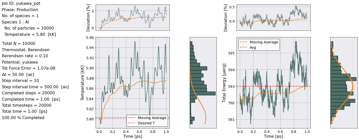
for i, lbl in zip(range(2), ["egs", "yukawa"]):
    # Get a new seed
    seed = rg.integers(0, 15198)

    args = {
        "Parameters": {"rand_seed": seed}, # define a new rand_seed for each simulation
        "Potential": {"type": lbl},
        "IO":   # Store all simulations' data in simulations_dir,
                # but save the dumps in different subfolders (job_dir)
            {
                "simulations_dir": 'SMT',
                "job_dir": "{}_pot".format(lbl),
                "verbose": False # This is so not to print to screen for every run
            },
    }

    # Run the simulation.
    sim = Simulation(input_file)
    sim.setup(read_yaml=True, other_inputs=args)
    sim.run()
    # Calculate RDF, SSF, Diffusion the simulation.
    pop = PostProcess(input_file)
    pop.setup(read_yaml=True, other_inputs=args)
    pop.parameters.verbose = True     # This is for printing informations about observables, and make plots.
    # FYI. this will be a little crowded
    pop.run()

Radial Distribution Function Calculation Time: 0 sec 2 msec 51 usec 255 nsec

Calculating n(k,t) for slice 0/1.

Calculating S(k) ...

Static Structure Factor Calculation Time: 0 sec 232 msec 461 usec 891 nsec

Radial Distribution Function Calculation Time: 0 sec 1 msec 969 usec 546 nsec

Calculating n(k,t) for slice 0/1.

Calculating S(k) ...

Static Structure Factor Calculation Time: 0 sec 24 msec 969 usec 611 nsec

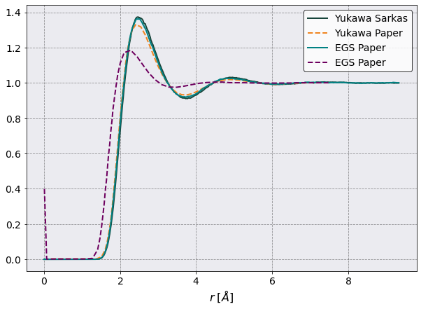
Radial Distribution Function

# Here is where I compare the two methods.
egs_data = pd.read_csv('SMT/egs_pot/PostProcessing/RadialDistributionFunction/Production/RadialDistributionFunction_egs_pot.csv', index_col = False)
yukawa_data = pd.read_csv('SMT/yukawa_pot/PostProcessing/RadialDistributionFunction/Production/RadialDistributionFunction_yukawa_pot.csv', index_col = False)

# Paper data
smt_data = np.loadtxt('egs.csv', delimiter=',' )
ysmt_data = np.loadtxt('yukawa.csv', delimiter=',' )

# make the plot
fig, ax = plt.subplots(1,1, figsize=(10,7))

ax.plot(yukawa_data['Distance'] * 1e8, yukawa_data['Al-Al RDF'], label = 'Yukawa Sarkas')
ax.plot(ysmt_data[:,0], ysmt_data[:,1], '--', label = 'Yukawa Paper')

ax.plot(egs_data['Distance'] * 1e8, egs_data['Al-Al RDF'], label = 'EGS Paper')
ax.plot(smt_data[:,0], smt_data[:,1], '--', label = 'EGS Paper')

ax.legend()
ax.set( xlabel = r'$r \; [ \AA] $')

[Text(0.5, 0, '$r \\; [ \\AA] $')]

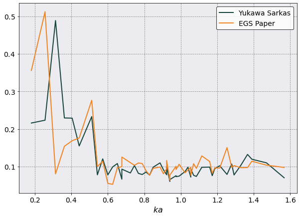
Static Structure Function

# Here is where I compare the two methods.
egs_data = pd.read_csv('SMT/egs_pot/PostProcessing/StaticStructureFunction/Production/StaticStructureFunction_egs_pot.csv', index_col=False)
yukawa_data = pd.read_csv('SMT/yukawa_pot/PostProcessing/StaticStructureFunction/Production/StaticStructureFunction_yukawa_pot.csv', index_col=False)

# Paper data
# smt_data = np.loadtxt('egs.csv', delimiter=',' )
# ysmt_data = np.loadtxt('yukawa.csv', delimiter=',' )

# make the plot
fig, ax = plt.subplots(1,1, figsize=(10,7))

ax.plot(yukawa_data['ka values'] , yukawa_data['Al-Al SSF'], label = 'Yukawa Sarkas')
# ax.plot(ysmt_data[:,0], ysmt_data[:,1], '--', label = 'Yukawa Paper')

ax.plot(egs_data['ka values'] , egs_data['Al-Al SSF'], label = 'EGS Paper')
# ax.plot(smt_data[:,0], smt_data[:,1], '--', label = 'EGS Paper')

ax.legend()
ax.set( xlabel = r'$ka$')

[Text(0.5, 0, '$ka$')]