
One Component Plasma (OCP)
Content
One Component Plasma (OCP)#
Oh the good ol’ OCP. The YAML input file can be found at input_file and this notebook at notebook.
[1]:
# Import the usual libraries
%pylab
%matplotlib inline

import os
plt.style.use('MSUstyle')

import pandas as pd
pd.options.display.max_columns = 15

# Import sarkas
from sarkas.processes import Simulation, PostProcess, PreProcess


# Create the file path to the YAML input file
input_file_name = os.path.join('input_files', 'coulomb_cgs.yaml')
Using matplotlib backend: Qt5Agg
Populating the interactive namespace from numpy and matplotlib
PreProcessing#
The following code is commented out since the simulation has been run before. We leave it here so that it is easy to copy and paste in your notebook.
[2]:
# preproc = PreProcess(input_file_name)
# preproc.setup(read_yaml=True)
# preproc.run(pppm_estimate=True)
Simulation#
The following code is commented out since the simulation has been run before. We leave it here so that it is easy to copy and paste in your notebook.
[3]:
# sim = Simulation(input_file_name)
# sim.setup(read_yaml=True)
# sim.run()
PostProcessing#
[4]:
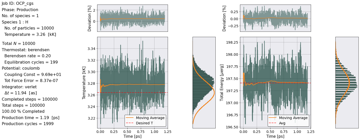
postproc = PostProcess(input_file_name)
postproc.setup(read_yaml=True)

postproc.therm.setup(postproc.parameters)
postproc.therm.temp_energy_plot(postproc)
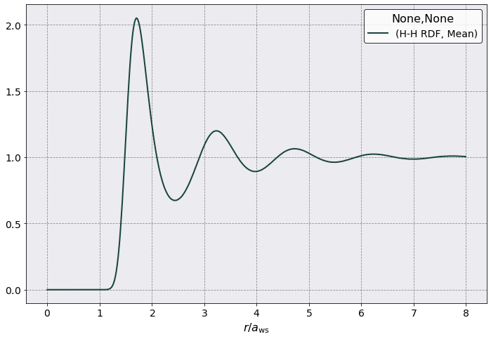
Radial Distribution Function#
[5]:
postproc.rdf.setup(postproc.parameters)
postproc.rdf.compute()
Radial Distribution Function Calculation Time: 0 sec 54 msec 472 usec 443 nsec
[6]:
postproc.rdf.plot(scaling = postproc.rdf.a_ws,
                  y = ("H-H RDF", "Mean"),
                  xlabel = r'$r/a_{\rm ws}$')
[6]:
<AxesSubplot:xlabel='$r/a_{\\rm ws}$'>
Calculate the Pressure from the RDF
[7]:
n_beta =  postproc.therm.beta / ( postproc.parameters.total_num_ptcls)
nkT, u_h, u_c, p_h, p_c = postproc.therm.compute_from_rdf(postproc.rdf, postproc.potential)
print('The excess pressure is = {:.4e} / (n k_B T)'.format(u_c[0] * n_beta ))
The excess pressure is = -8.2438e+01 / (n k_B T)
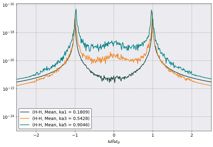
Dynamic Structure Factor#
[8]:
from sarkas.tools.observables import DynamicStructureFactor

dsf = DynamicStructureFactor()
dsf.max_ka_value = 10
dsf.angle_averaging = 'principal_axis'
dsf.no_slices = 4
dsf.setup(postproc.parameters)
dsf.pretty_print()
====================== Dynamic Structure Factor ======================

k wavevector information saved in:
 Simulations/OCP_cgs/PostProcessing/k_space_data/k_arrays.npz
n(k,t) data saved in:
 Simulations/OCP_cgs/PostProcessing/k_space_data/nkt.h5
Data saved in:
 Simulations/OCP_cgs/PostProcessing/DynamicStructureFactor/Production/DynamicStructureFactor_OCP_cgs.h5
Data accessible at: self.k_list, self.k_counts, self.ka_values, self.frequencies, self.dataframe

Frequency Space Parameters:
        No. of slices = 1
        No. dumps per slice = 50001
        Frequency step dw = 2 pi (no_slices * prod_dump_step)/(production_steps * dt)
        dw = 0.0031 w_p = 5.2642e+12 [rad/s]
        Maximum Frequency w_max = 2 pi /(prod_dump_step * dt)
        w_max = 78.5487 w_p = 1.3161e+17 [rad/s]


Wavevector parameters:
Smallest wavevector k_min = 2 pi / L = 3.9 / N^(1/3)
k_min = 0.1809 / a_ws = 3.4252e+07 [1/cm]

Angle averaging choice: principal_axis
        Maximum k harmonics = n_x, n_y, n_z = 55, 55, 55
        Largest wavector k_max = k_min * n_x
        k_max = 9.9505 / a_ws = 1.8839e+09 [1/cm]

Total number of k values to calculate = 165
No. of unique ka values to calculate = 55
[9]:
dsf.parse()
[10]:
dsf.dataframe
[10]:
| H-H | |||||||||||||||
|---|---|---|---|---|---|---|---|---|---|---|---|---|---|---|---|
| Mean | ... | Std | |||||||||||||
| Frequencies | ka1 = 0.1809 | ka2 = 0.3618 | ka3 = 0.5428 | ka4 = 0.7237 | ka5 = 0.9046 | ka6 = 1.0855 | ... | ka49 = 8.8650 | ka50 = 9.0459 | ka51 = 9.2269 | ka52 = 9.4078 | ka53 = 9.5887 | ka54 = 9.7696 | ka55 = 9.9505 | |
| 0 | -1.316086e+17 | 4.879578e-25 | 1.472862e-25 | 2.390647e-25 | 2.450585e-25 | 7.464846e-25 | 1.143595e-24 | ... | 3.108407e-22 | 2.788587e-22 | 1.524755e-22 | 2.245008e-22 | 5.311622e-23 | 2.032679e-22 | 1.299485e-22 |
| 1 | -1.315876e+17 | 4.879578e-25 | 1.472866e-25 | 2.390647e-25 | 2.450578e-25 | 7.464843e-25 | 1.143596e-24 | ... | 3.108408e-22 | 2.788584e-22 | 1.524759e-22 | 2.245011e-22 | 5.311582e-23 | 2.032684e-22 | 1.299482e-22 |
| 2 | -1.315665e+17 | 4.879578e-25 | 1.472870e-25 | 2.390648e-25 | 2.450572e-25 | 7.464841e-25 | 1.143597e-24 | ... | 3.108409e-22 | 2.788580e-22 | 1.524764e-22 | 2.245014e-22 | 5.311542e-23 | 2.032690e-22 | 1.299479e-22 |
| 3 | -1.315455e+17 | 4.879579e-25 | 1.472874e-25 | 2.390650e-25 | 2.450566e-25 | 7.464840e-25 | 1.143599e-24 | ... | 3.108411e-22 | 2.788577e-22 | 1.524769e-22 | 2.245017e-22 | 5.311503e-23 | 2.032697e-22 | 1.299476e-22 |
| 4 | -1.315244e+17 | 4.879581e-25 | 1.472878e-25 | 2.390651e-25 | 2.450560e-25 | 7.464840e-25 | 1.143600e-24 | ... | 3.108413e-22 | 2.788575e-22 | 1.524774e-22 | 2.245021e-22 | 5.311465e-23 | 2.032703e-22 | 1.299474e-22 |
| ... | ... | ... | ... | ... | ... | ... | ... | ... | ... | ... | ... | ... | ... | ... | ... |
| 12495 | 1.315033e+17 | 4.879589e-25 | 1.472846e-25 | 2.390648e-25 | 2.450623e-25 | 7.464874e-25 | 1.143593e-24 | ... | 3.108409e-22 | 2.788611e-22 | 1.524735e-22 | 2.245000e-22 | 5.311834e-23 | 2.032654e-22 | 1.299503e-22 |
| 12496 | 1.315244e+17 | 4.879585e-25 | 1.472849e-25 | 2.390647e-25 | 2.450615e-25 | 7.464866e-25 | 1.143593e-24 | ... | 3.108408e-22 | 2.788606e-22 | 1.524738e-22 | 2.245001e-22 | 5.311790e-23 | 2.032658e-22 | 1.299499e-22 |
| 12497 | 1.315455e+17 | 4.879583e-25 | 1.472852e-25 | 2.390646e-25 | 2.450607e-25 | 7.464860e-25 | 1.143593e-24 | ... | 3.108407e-22 | 2.788601e-22 | 1.524742e-22 | 2.245002e-22 | 5.311747e-23 | 2.032663e-22 | 1.299495e-22 |
| 12498 | 1.315665e+17 | 4.879581e-25 | 1.472855e-25 | 2.390646e-25 | 2.450599e-25 | 7.464854e-25 | 1.143594e-24 | ... | 3.108406e-22 | 2.788596e-22 | 1.524746e-22 | 2.245004e-22 | 5.311705e-23 | 2.032668e-22 | 1.299492e-22 |
| 12499 | 1.315876e+17 | 4.879579e-25 | 1.472859e-25 | 2.390646e-25 | 2.450592e-25 | 7.464850e-25 | 1.143595e-24 | ... | 3.108407e-22 | 2.788591e-22 | 1.524750e-22 | 2.245006e-22 | 5.311663e-23 | 2.032673e-22 | 1.299488e-22 |
12500 rows × 111 columns
[11]:
ax = dsf.plot(scaling = dsf.total_plasma_frequency,
         y = [("H-H","Mean", "ka1 = 0.1809"), ("H-H","Mean", "ka3 = 0.5428"), ("H-H","Mean", "ka5 = 0.9046")],
         xlabel = r'$\omega/\omega_p$',
         xlim = (-2.5, 2.5),
        logy = True)
ax.legend()
[11]:
<matplotlib.legend.Legend at 0x7fdb2adc8d90>
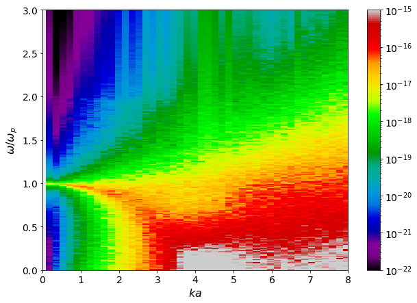
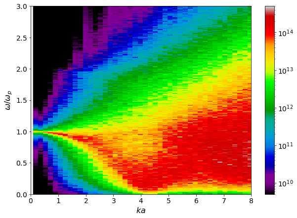
Collective Mode Dispersion#
[12]:
w = dsf.dataframe[(" "," ","Frequencies")]/ dsf.total_plasma_frequency

ka_mesh, w_mesh = np.meshgrid(dsf.ka_values, w)

Skw = dsf.dataframe[("H-H", "Mean")]
fig, ax = plt.subplots(1,1)
pc = ax.pcolormesh(ka_mesh, w_mesh, Skw,
                   shading = 'auto',
                   norm = mpl.colors.LogNorm(vmin = 1e-22, vmax = 1e-15),
                   cmap='nipy_spectral')
ax.set(ylim = (0,3),
       xlim = (0,8),
       xlabel = r'$ka$',
       ylabel = r'$\omega/\omega_p$')
plt.colorbar(pc)
[12]:
<matplotlib.colorbar.Colorbar at 0x7fdb2b62e490>
[13]:
from sarkas.tools.observables import CurrentCorrelationFunction

ccf = CurrentCorrelationFunction()
ccf.max_ka_value = 10
ccf.angle_averaging = 'principal_axis'
ccf.no_slices = 4
ccf.setup(postproc.parameters)
ccf.pretty_print()
==================== Current Correlation Function ====================

k wavevector information saved in:
 Simulations/OCP_cgs/PostProcessing/k_space_data/k_arrays.npz
v(k,t) data saved in:
 Simulations/OCP_cgs/PostProcessing/k_space_data/vkt.h5
Data saved in:
Simulations/OCP_cgs/PostProcessing/CurrentCorrelationFunction/Production/CurrentCorrelationFunction_OCP_cgs.h5
Data accessible at: self.k_list, self.k_counts, self.ka_values, self.frequencies,
         self.dataframe

Frequency Space Parameters:
        No. of slices = 4
        No. dumps per slice = 12500
        Frequency step dw = 2 pi (no_slices * prod_dump_step)/(production_steps * dt)
        dw = 0.0126 w_p = 2.1057e+13 [rad/s]
        Maximum Frequency w_max = 2 pi /(prod_dump_step * dt)
        w_max = 78.5487 w_p = 1.3161e+17 [rad/s]


Wavevector parameters:
Smallest wavevector k_min = 2 pi / L = 3.9 / N^(1/3)
k_min = 0.1809 / a_ws = 3.4252e+07 [1/cm]

Angle averaging choice: principal_axis
        Maximum k harmonics = n_x, n_y, n_z = 55, 55, 55
        Largest wavector k_max = k_min * n_x
        k_max = 9.9505 / a_ws = 1.8839e+09 [1/cm]

Total number of k values to calculate = 165
No. of unique ka values to calculate = 55
[14]:
# ccf.compute()
ccf.parse()
[15]:
ccf.dataframe
[15]:
| Longitudinal | ... | Transverse | |||||||||||||
|---|---|---|---|---|---|---|---|---|---|---|---|---|---|---|---|
| H-H | ... | H-H | |||||||||||||
| Mean | ... | Std | |||||||||||||
| ka1 = 0.1809 | ka2 = 0.3618 | ka3 = 0.5428 | ka4 = 0.7237 | ka5 = 0.9046 | ka6 = 1.0855 | ... | ka49 = 8.8650 | ka50 = 9.0459 | ka51 = 9.2269 | ka52 = 9.4078 | ka53 = 9.5887 | ka54 = 9.7696 | ka55 = 9.9505 | ||
| Frequencies | NaN | NaN | NaN | NaN | NaN | NaN | ... | NaN | NaN | NaN | NaN | NaN | NaN | NaN | |
| 0 | -1.316086e+17 | 297360.958948 | 550841.305756 | 741502.511222 | 1.016348e+06 | 1.514701e+06 | 2.271082e+06 | ... | 7.750616e+07 | 5.889132e+07 | 9.418742e+07 | 5.108627e+07 | 7.961882e+07 | 1.341673e+08 | 2.069157e+08 |
| 1 | -1.315876e+17 | 297360.776416 | 550842.124002 | 741502.375627 | 1.016346e+06 | 1.514700e+06 | 2.271084e+06 | ... | 7.750625e+07 | 5.889105e+07 | 9.418693e+07 | 5.108631e+07 | 7.961854e+07 | 1.341673e+08 | 2.069154e+08 |
| 2 | -1.315665e+17 | 297360.647363 | 550843.139040 | 741502.337668 | 1.016345e+06 | 1.514699e+06 | 2.271087e+06 | ... | 7.750636e+07 | 5.889082e+07 | 9.418642e+07 | 5.108637e+07 | 7.961826e+07 | 1.341674e+08 | 2.069150e+08 |
| 3 | -1.315455e+17 | 297360.545013 | 550844.190843 | 741502.511066 | 1.016343e+06 | 1.514697e+06 | 2.271090e+06 | ... | 7.750648e+07 | 5.889055e+07 | 9.418595e+07 | 5.108642e+07 | 7.961800e+07 | 1.341674e+08 | 2.069148e+08 |
| 4 | -1.315244e+17 | 297360.479300 | 550845.235350 | 741502.714944 | 1.016342e+06 | 1.514696e+06 | 2.271093e+06 | ... | 7.750661e+07 | 5.889032e+07 | 9.418548e+07 | 5.108648e+07 | 7.961773e+07 | 1.341676e+08 | 2.069145e+08 |
| ... | ... | ... | ... | ... | ... | ... | ... | ... | ... | ... | ... | ... | ... | ... | ... |
| 12495 | 1.315033e+17 | 297362.379926 | 550837.777453 | 741504.525321 | 1.016359e+06 | 1.514712e+06 | 2.271074e+06 | ... | 7.750583e+07 | 5.889277e+07 | 9.419012e+07 | 5.108613e+07 | 7.962035e+07 | 1.341672e+08 | 2.069178e+08 |
| 12496 | 1.315244e+17 | 297362.038693 | 550838.295542 | 741504.077521 | 1.016357e+06 | 1.514710e+06 | 2.271075e+06 | ... | 7.750587e+07 | 5.889246e+07 | 9.418956e+07 | 5.108616e+07 | 7.962006e+07 | 1.341671e+08 | 2.069173e+08 |
| 12497 | 1.315455e+17 | 297361.694330 | 550838.950322 | 741503.502435 | 1.016354e+06 | 1.514707e+06 | 2.271076e+06 | ... | 7.750592e+07 | 5.889217e+07 | 9.418901e+07 | 5.108617e+07 | 7.961974e+07 | 1.341672e+08 | 2.069169e+08 |
| 12498 | 1.315665e+17 | 297361.427877 | 550839.707170 | 741503.103073 | 1.016352e+06 | 1.514705e+06 | 2.271078e+06 | ... | 7.750600e+07 | 5.889188e+07 | 9.418847e+07 | 5.108619e+07 | 7.961942e+07 | 1.341672e+08 | 2.069165e+08 |
| 12499 | 1.315876e+17 | 297361.173344 | 550840.413166 | 741502.795738 | 1.016350e+06 | 1.514703e+06 | 2.271080e+06 | ... | 7.750607e+07 | 5.889160e+07 | 9.418794e+07 | 5.108622e+07 | 7.961910e+07 | 1.341672e+08 | 2.069160e+08 |
12500 rows × 221 columns
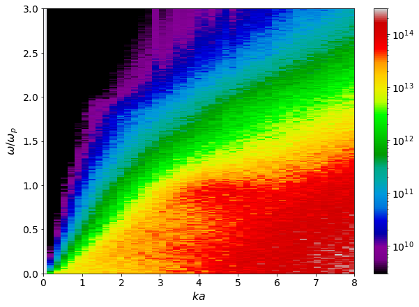
[16]:
w = dsf.dataframe[(" "," ","Frequencies")]/ ccf.total_plasma_frequency

ka_mesh, w_mesh = np.meshgrid(dsf.ka_values, w)

Lkw = ccf.dataframe[("Longitudinal", "H-H", "Mean")]
fig, ax = plt.subplots(1,1)
pc = ax.pcolormesh(ka_mesh, w_mesh, Lkw,
                   shading = 'auto',
                   norm = mpl.colors.LogNorm(vmin = 0.5e10, vmax = 0.5e15),
                   cmap='nipy_spectral')
ax.set(ylim = (0,3),
       xlim = (0,8),
       xlabel = r'$ka$',
       ylabel = r'$\omega/\omega_p$')
plt.colorbar(pc)
[16]:
<matplotlib.colorbar.Colorbar at 0x7fdb2f889610>
[17]:
w = dsf.dataframe[(" "," ","Frequencies")]/ ccf.total_plasma_frequency

ka_mesh, w_mesh = np.meshgrid(dsf.ka_values, w)

Lkw = ccf.dataframe[("Transverse", "H-H", "Mean")]
fig, ax = plt.subplots(1,1)
pc = ax.pcolormesh(ka_mesh, w_mesh, Lkw,
                   shading = 'auto',
                   norm = mpl.colors.LogNorm(vmin = 3e9, vmax = 3e14),
                   cmap='nipy_spectral')
ax.set(ylim = (0,3),
       xlim = (0,8),
       xlabel = r'$ka$',
       ylabel = r'$\omega/\omega_p$')
plt.colorbar(pc)
[17]:
<matplotlib.colorbar.Colorbar at 0x7fdb2ae4f290>
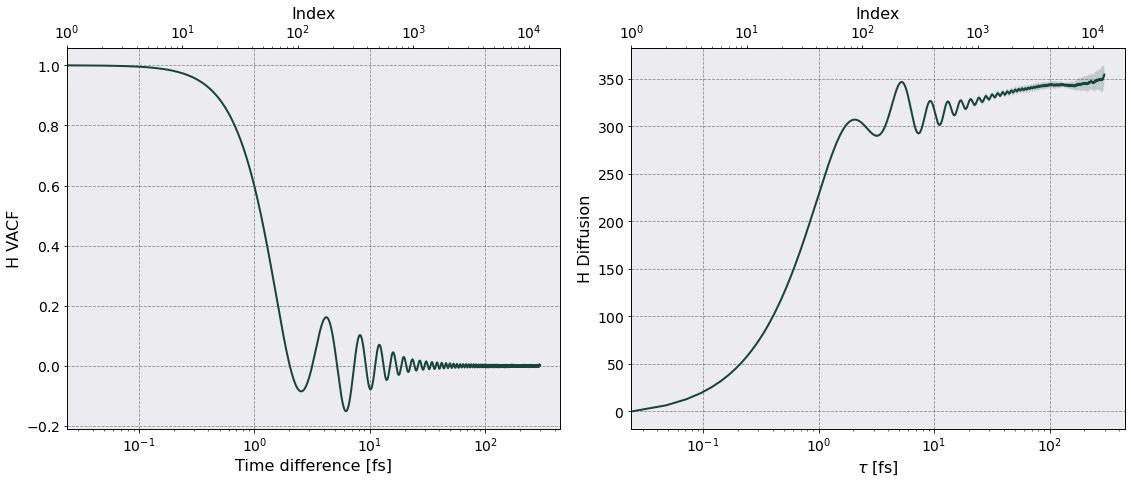
Diffusion#
Diffusion is calculated from the integral of the velocity autocorrelation function, \(\left \langle \bar{\mathbf v} (t) \cdot \bar{\mathbf v}(0) \right \rangle\),
\begin{equation} D = \frac{1}{3} \int_0^{\tau} dt \, \left \langle \bar{\mathbf v} (t) \cdot \bar{\mathbf v}(0) \right \rangle \end{equation}
where \(\bar{\mathbf v}\) is the particle-averaged velocity.
[18]:
from sarkas.tools.observables import VelocityAutoCorrelationFunction
from sarkas.tools.transport import TransportCoefficients
[19]:
vacf = VelocityAutoCorrelationFunction()
vacf.setup(postproc.parameters, no_slices=4)
[20]:
vacf.parse()
[21]:
tc = TransportCoefficients(postproc.parameters, no_slices = 4)
tc.diffusion(vacf, plot=True)
======================= Diffusion Coefficient ========================

Data saved in:
 Simulations/OCP_cgs/PostProcessing/TransportCoefficients/Production/Diffusion_OCP_cgs.h5
Simulations/OCP_cgs/PostProcessing/TransportCoefficients/Production/Diffusion_slices_OCP_cgs.h5

No. of slices = 4
No. dumps per slice = 6250
Time interval of autocorrelation function = 2.9838e-13 [s] ~ 499 w_p T
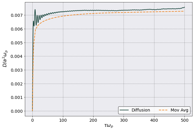
[22]:
rescaling = 1.0/vacf.total_plasma_frequency/vacf.a_ws**2
fig, ax = plt.subplots(1,1, figsize=(10,7))
ax.plot(tc.diffusion_df["Time"].iloc[:,0]*vacf.total_plasma_frequency,
        tc.diffusion_df[("H Diffusion","Mean")] * rescaling,
       label = r'Diffusion')

ax.plot(tc.diffusion_df["Time"].iloc[:,0]*vacf.total_plasma_frequency,
        tc.diffusion_df[("H Diffusion","Mean")].expanding().mean() * rescaling,
        ls = '--', label = r'Mov Avg')

ax.legend(ncol = 2)
ax.set(xlabel = r"$\tau \omega_p$",ylabel = r" $D/a^2 \omega_p$")
[22]:
[Text(0.5, 0, '$\\tau \\omega_p$'), Text(0, 0.5, ' $D/a^2 \\omega_p$')]
[ ]: